Chapter 09 – Short-Term Profit Planning: Cost-Volume-Profit (CVP) Analysis
9-24 Cost Planning: The Cost of an MBA; Time Value of Money (20
minutes)
Using the present value factor (4.212) for an annuity for five years at 6%
shows that the present value of $23,742 per year is $100,000 ($100,000 ÷
4.212); this means that for the student a current payment (at one point in
time in this simplified example) of $100,000 is equivalent to receiving a
Note that the cost of the program includes the foregone pre-MBA salary,
and for students at prestigious programs like School B, the pre-MBA
salaries are relatively high. So the increase in salary post-MBA does not
show the degree of “bump” that is seen in other schools. Also, the
calculation above does not reflect the opportunity that might attract a new
MBA to a company, apart from the pay offer. For example, BusinessWeek
provides a listing of its Top-50 Employers, based on surveys of students,
college placement personnel, and the employers themselves. As of
September 2008, the Big-4 public accounting firms, Goldman Sachs,
Google, Marriott, Lockheed Martin, IBM and JPMorgan/Chase lead the list.
Another Business Week survey shows the cost and increase in pay for 20
well-known U.S. universities. Brigham Young University is shown as the top
value with a high ratio of pay increase to cost.
A Wall Street Journal ranking of the return on investment for top executive
MBA programs, based on tuition costs and projected salary, shows
surprising results, among them that the top five programs are at public
Universities; the highest-ranked program, Texas A&M University, produced
a 243% return on investment.
Source: “The High Price of Admission,” BusinessWeek, October 23, 2006,
p. 60. Also: “Fifty Employers with the Right Stuff,” BusinessWeek,
September 15, 2008, p. 39; Alina Dizik, “Ranking the Returns on Executive
MBAs,” The Wall Street Journal, December 10, 2008, p D1.
9-10
Education.
Chapter 09 – Short-Term Profit Planning: Cost-Volume-Profit (CVP) Analysis
9-25 Cost Planning; Gasoline Prices (20-25 minutes)
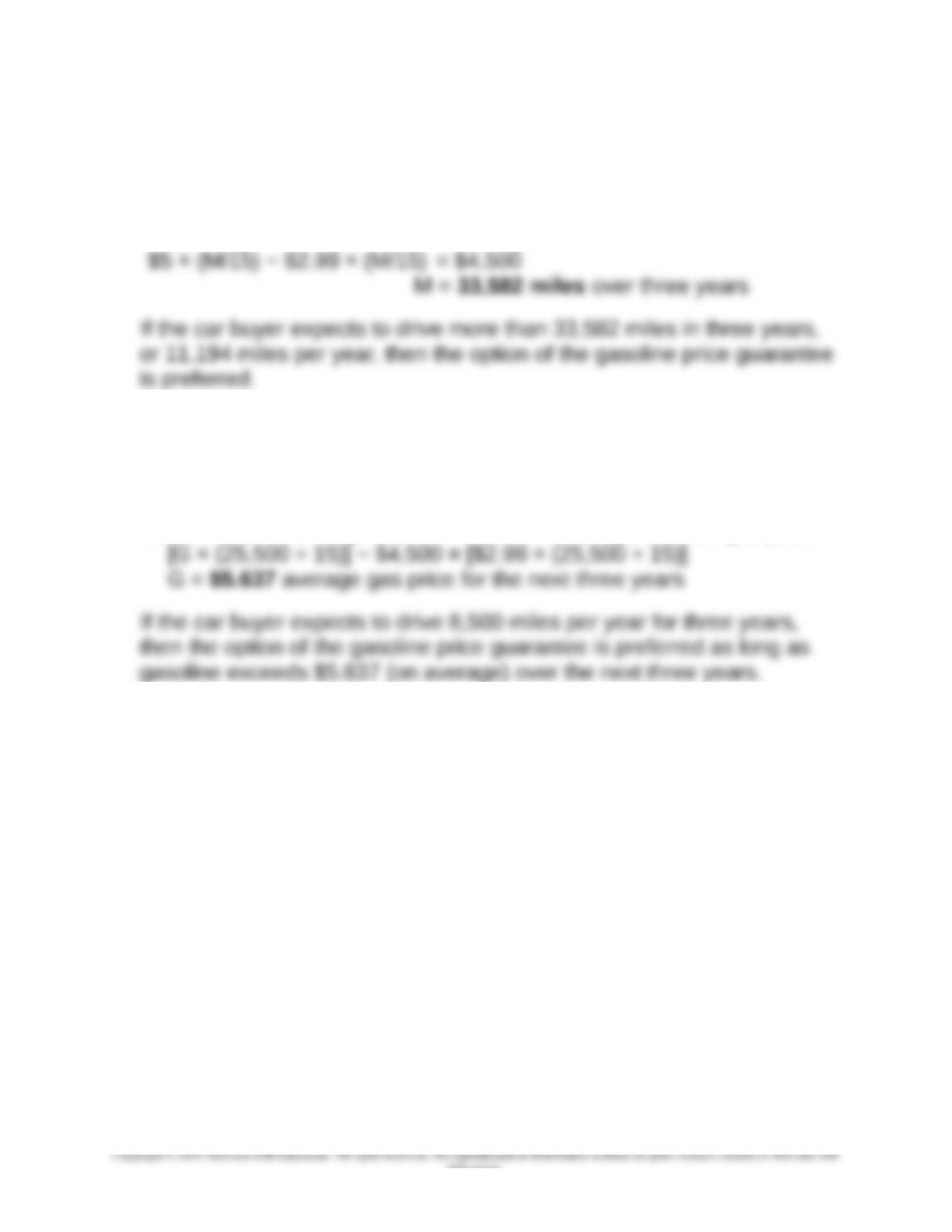
1. Solve for the indifference point in miles (M) where 15 is the mpg, $2.99 is
the guarantee price, and $5.00 is the expected price:
Savings for the guarantee = Savings for the discount
2. Solve for the indifference point in gasoline price (G) where 15 is the
mpg, and $2.99 is the guaranteed price and 8,500 is the expected
annual mileage (8,500 × 3 years = 25,500 miles for three years):
Total cost without the guarantee = Total cost with guaranteed gas price
3. Some important decision factors include:
Do I need a new car, or should I save the money by fixing up my
present car, including a tune up and new tires which could help
improve gas mileage
Will gasoline prices fall? (as of December 1, 2008, gasoline prices
had fallen to below $2.00 per gallon, and Chrysler’s promotion would
have made no sense; but gasoline had increased to $2.60 per gallon
in June of 2009)
Should I look to use mass transit and reduce the gas I use in that
way?
Should I look for a vehicle which gets much better gas mileage than
the one described?
If in an urban area or where it is available, should I use car-share
programs?
9-11
Education.
Chapter 09 – Short-Term Profit Planning: Cost-Volume-Profit (CVP) Analysis
9-26 The Role of Income Taxes (20 minutes)
1. Pre-tax income = After-tax income ÷ (1 – t)
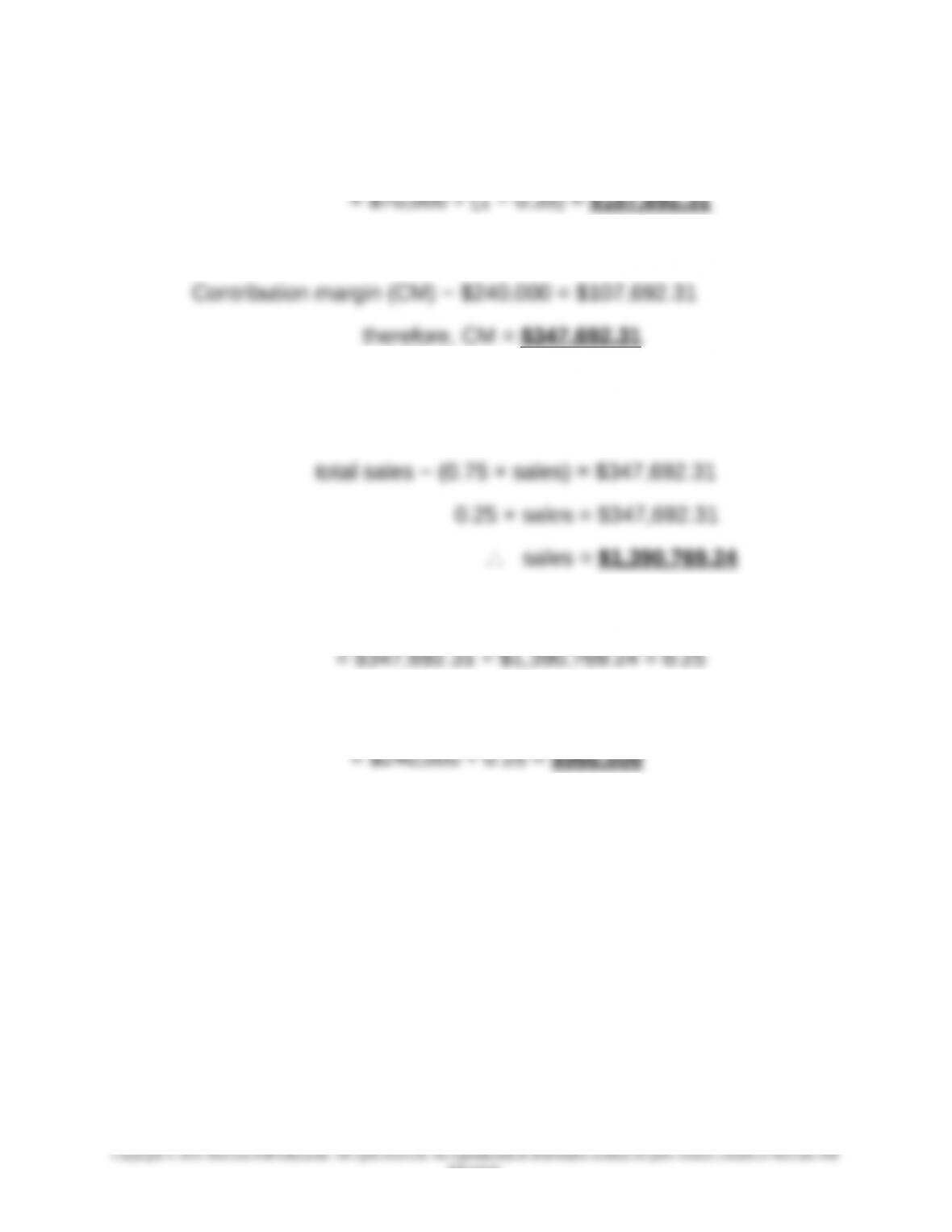
2. Contribution margin − fixed costs = before tax profit
3. total sales − total variable cost = total contribution margin (CM)
total sales – (variable cost ratio × sales) = $347,692.31
4. Contribution margin ratio (CMR) = CM ÷ Sales
= $347,692.31 ÷ $1,390,769.24 = 0.25
Breakeven point = fixed costs (F) ÷ CMR
9-12
Education.
Chapter 09 – Short-Term Profit Planning: Cost-Volume-Profit (CVP) Analysis
9-27 CVP Analysis with IncomeTaxes (20-25 minutes)
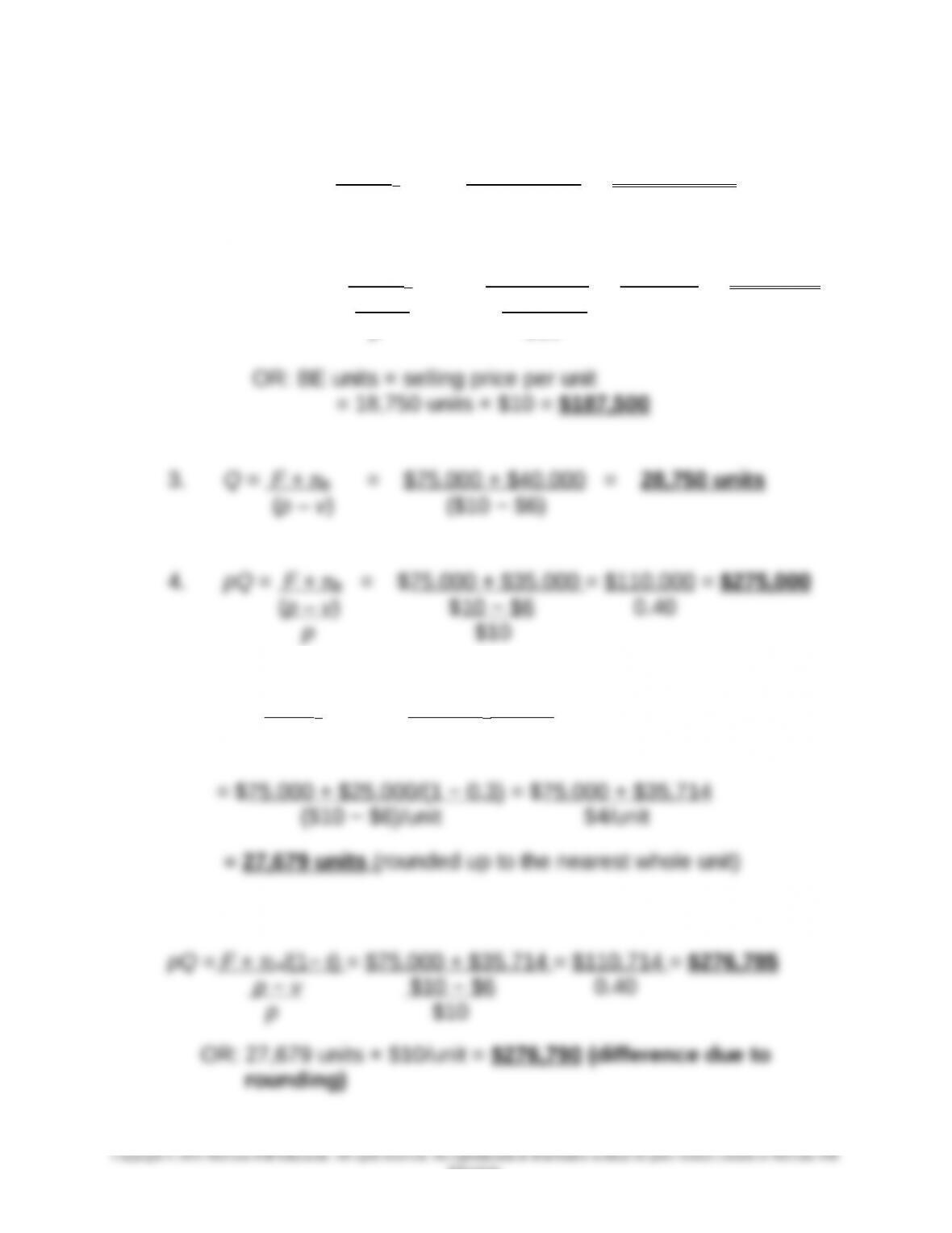
1. BE units = F + π B = $75,000 + 0 = 18,750 units
(p – v) ($10 − $6)/unit
2. BE dollars = F + π B = $75,000 + 0 = $75,000 = $187,500
(p – v ) $10 − $6 0.40
p $10
5. Q = F + π B = F + π A/(1 − t )
(p – v) (p – v)
Using the contribution margin ratio (CMR):
9-13
Education.
Chapter 09 – Short-Term Profit Planning: Cost-Volume-Profit (CVP) Analysis
9-28 Cost Planning: High-End Copiers (20-25 minutes)
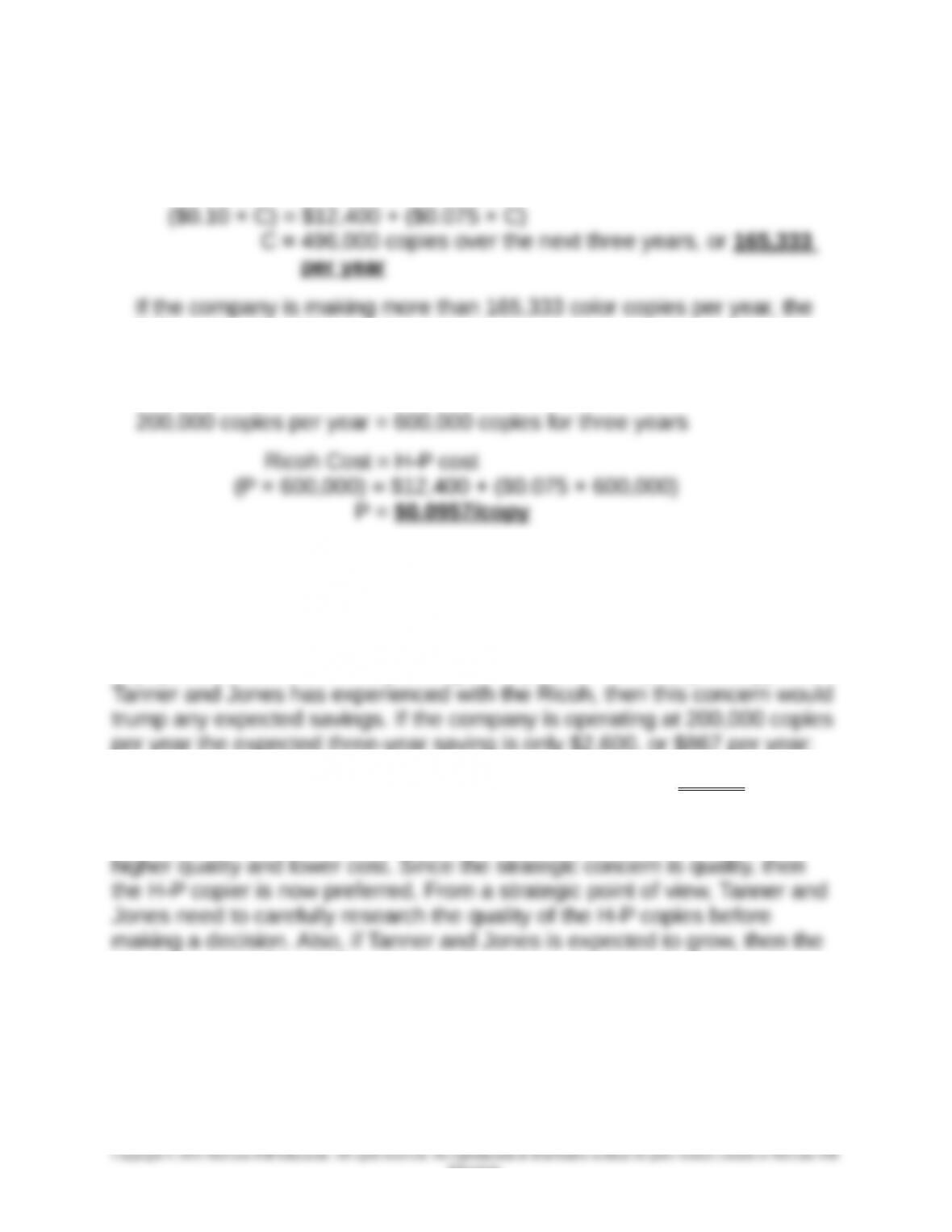
1. The breakeven number of copies (C) can be determined as follows:
Ricoh Cost = H-P Cost
H-P copier should lead to lower total costs.
2. The breakeven price (P) can be determined as follows:
Tanner and Jones should be able to negotiate with Ricoh to reduce its
color copy price from $0.10 to perhaps $0.096
3. Since Tanner and Jones competes on quality and service, it is critical
that the company has a reliable and very high quality color copier. If there is
any question that the H-P copier might not provide the quality of copy that
per year the expected three-year saving is only $2,600, or $867 per year:
($0.10 × 600,000) − $12,400 − ($0.075 × 600,000) = $2,600
This small amount of saving should not justify the risk of unknown color
quality. On the other hand, it is possible that the H-P copier would deliver
attractiveness of the H-P copier also increases, because the lower price
per copy now applies to a larger number of copies.
Source: Christopher Lawton, “H-P Begins Push Into High-End Copiers,”
The Wall Street Journal, April 24, 2007.
9-14
Education.
Chapter 09 – Short-Term Profit Planning: Cost-Volume-Profit (CVP) Analysis
9-29 Margin of Safety (MOS) (20 minutes)
1. First, calculate the breakeven point, using the contribution margin ratio
(CMR), as follows:
CMR = Contribution Margin ÷ Sales = $227,500 ÷ $650,000 = 0.35
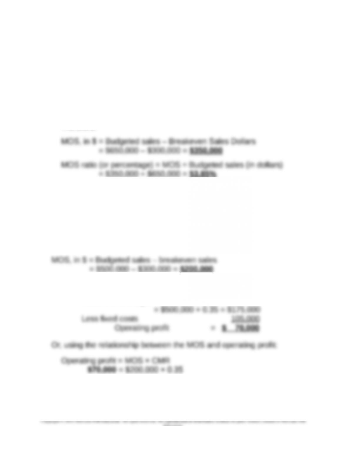
Breakeven in dollars = Fixed Costs ÷ CMR = $105,000 ÷ 0.35 =
$300,000
Therefore:
2. The MOS and related MOS ratio (or, percentage) are rough measures of
operating risk. They indicate the amount by which sales could fall—
either in absolute dollars or in percentage terms—before losses are
incurred.
3. If sales fall to $500,000, the breakeven point will remain the same, but
the MOS will change:
Operating profit:
Contribution margin = Sales $ × CMR
9-15
Education.

Chapter 09 – Short-Term Profit Planning: Cost-Volume-Profit (CVP) Analysis
9-29 (Continued)
Why this works:
Operating profit = MOS × CMR
= (Expected Sales − Breakeven) × CMR
(Note: by definition, breakeven in sales dollars × CMR = fixed costs; i.e., at
the breakeven point there is just enough contribution margin generated to
cover total fixed costs, F)
9-16
Chapter 09 – Short-Term Profit Planning: Cost-Volume-Profit (CVP) Analysis
9-30 Degree of Operating Leverage (DOL) (25 minutes)
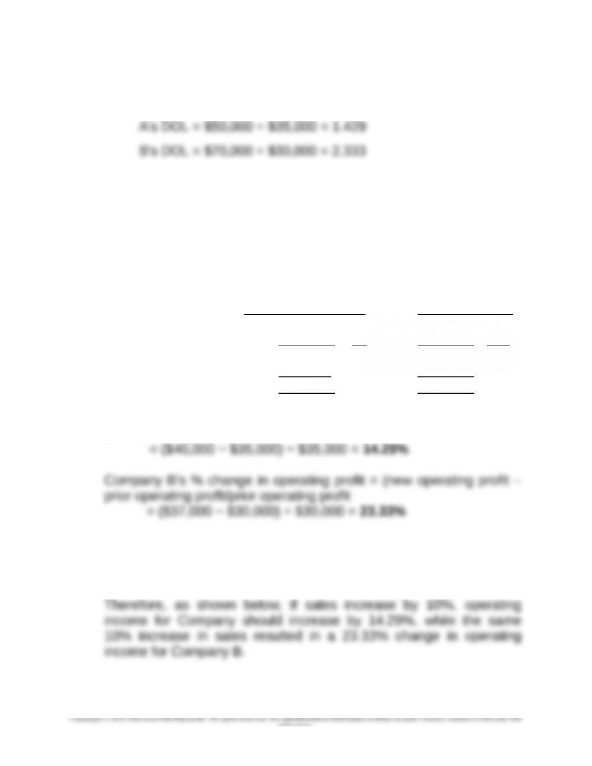
1. DOL = contribution margin ÷ operating profit
If sales increase, company B will benefit more. Company B has a
higher proportion of fixed costs in relation to variable costs; therefore
it has a higher operating leverage than does Company A. The degree
of operating leverage (DOL) is a measure, at a specific level of sales,
of how a percentage change in sales volume will affect profits. The
higher the operating leverage, the more sensitive profits are to
changes in sales volume.
2. Company A Company B
Amount % Amount %
Sales $110,000 100 $110,000 100
Less variable costs 55,000 50 33,000 30
Contribution margin $ 55,000 50 $ 77,000 70
Less fixed costs 15,000 40,000
Operating profit $ 40,000 $ 37,000
Company A’s % change in operating profit = (new operating profit –
prior operating profit)/prior operating profit
The above results are what we expected. The DOL tells us the
estimated % change in operating income for each percentage change
in sales. A DOL of 1.429 implies that the change in operating income
will be 1.429 times as large as the % change in sales volume.
9-17
Education.
Chapter 09 – Short-Term Profit Planning: Cost-Volume-Profit (CVP) Analysis
9-30 (Continued)
A’s % change in profits = DOL × % change in sales = 1.429 × 10% =
14.29%
3. Further interpretation of DOL—in what sense is DOL a measure of
risk? As indicated by the above responses, DOL measures how
sensitive operating profits are to changes in sales volume. If DOL is
high, then even small (%) changes in sales will lead to large (%)
changes in operating income. It is this magnification process that
captures what is called business or operating risk (as compared, for
example, to financial risk). As the level of operation changes (i.e., as
sales volume changes) so too does operating profit, both on the
9-18
Chapter 09 – Short-Term Profit Planning: Cost-Volume-Profit (CVP) Analysis
9-31 CVP Analysis, DOL, and Margin of Safety (40-45 minutes)
First, note that the DOL formula, at any sales volume level, Q, is written as:
Second, define the change in OI and the change in S with respect to the
break-even point (B/E), as follows:
DOLQ = ([OIX − OIB/E] /OIQ) ÷ ([SQ − SB/E]/SQ)
Third, since by definition OIB/E = 0, the above reduces to:
DOLQ = (OIQ/OIQ) ÷ ([SQ– SB/E]/SQ)
2. The above specification allows managers to see that operating leverage
and margin of sales are functionally related: the greater the relative
amount of fixed costs (F), the lower the safety margin (MOS) at any
given volume level, Q, and the higher the degree of operating leverage
(DOL).
9-19
Education.