Unlock document.
This document is partially blurred.
Unlock all pages and 1 million more documents.
Get Access

Chapter 09 - Short-Term Profit Planning: Cost-Volume-Profit (CVP) Analysis
Another analytical approach to sensitivity analysis is to express the factors of the CVP model as random
variables, and then to examine the outputs of the model probabilistically. This approach also has the benefit of
mathematical precision noted above, but it requires a certain expertise as well as certain potentially restrictive
assumptions. When the expertise is available and the assumptions can be fairly made, the probabilistic model
can be a very useful analysis tool for the manager.2 See also the lecture note below, “CVP Analysis with Non-
linear Cost and Revenue.”
Simulation
By simulation we mean the systematic "what if?" types of analyses that the manager can use to diagnose
potential problem areas before a project is undertaken. A direct and common approach for this type of
simulation is to use a spreadsheet. To illustrate, we have developed two spreadsheets (Exhibits 1 and 2) to
demonstrate the two different ways the simulation can be done. Exhibit 1 illustrates a pro-forma income
statement which incorporates all the factors of the CVP model (unit variable cost, fixed cost, price, desired
profit, quantity), and lets us observe the one-at-a-time changes of any of the individual factors on the others.
This spreadsheet would be very useful for the manager who wants to assess quickly and easily the potential
effects of forecast errors, of policy changes, of unexpected economic or competitive changes, and other
managerial issues.3
For example, the spreadsheet could be used to examine the effect on net income of a change in sales quantity
from 250 to 300 units. By inserting 300 in cell B7, the management accountant would see the spreadsheet
automatically recalculate contribution margin (now $12,000) and net income (now $7,000). Similar "what if?"
types of queries could be answered by inserting new values for variable cost, fixed cost, or any other cost
factor in the case. Part 2 of the spreadsheet shows summary cost-volume-profit information for the data given
in Part 1.
2 The probabilistic analysis of the CVP model is covered in the following articles: Hilliard, Jimmy E., and Robert A.
Leitch, "Breakeven Analysis of Alternatives under Uncertainty," Management Accounting (March 1977), pp. 53-57, and
Jaedicke, Robert K., and Alexander A. Robichek, "Cost-Volume-Profit Analysis Under Conditions of Uncertainty," The
Accounting Review (October 1964), pp. 917-926.
3 As noted earlier, the following reference could be consulted: Thomas E. McKee, “Using Excel to Perform Monte Carlo
Simulations,” Strategic Finance (December 2014), pp. 47-51.
9-11
Education.

Chapter 09 - Short-Term Profit Planning: Cost-Volume-Profit (CVP) Analysis
Exhibit 1: A Spreadsheet for Cost-Volume-Profit (CVP) Analysis
---------------------------A--------------------------B-------------------------------C------------
1 COST-VOLUME-PROFIT ANALYSIS
2 HOUSEHOLD FURNISHINGS, INC
3
4 PART 1: INCOME STATEMENT
5
6 REVENUES
7 SALES QUANTITY 250
8 SALES PRICE 75
9 TOTAL REVENUES 18,750
10
11 UNIT VARIABLE COSTS
12 MATERIALS
13 LABOR
14 SELLING COSTS
15 TOTAL UNIT VARIABLE COSTS 35
16 TOTAL VARIABLE COSTS 8,750
17 CONTRIBUTION MARGIN 10,000
18
19 FIXED COSTS
20 MANUFACTURING
21 SELLING
22 ADMINISTRATIVE
23 TOTAL FIXED COSTS 5,000
24
25 NET INCOME 5,000
26
27
28 PART 2: COST-VOLUME-PROFIT ANALYSIS
29
30
31 BREAKEVEN IN UNITS 125
32 BREAKEVEN IN $ 9,375
33
34 UNIT CONTRIBUTION MARGIN 40
35 CONTRIBUTION MARGIN RATIO 0.533
36
37 OPERATING LEVERAGE 3.75
38 MARGIN OF SAFETY 125 units
9-12
Education.

Chapter 09 - Short-Term Profit Planning: Cost-Volume-Profit (CVP) Analysis
The second spreadsheet (Exhibit 2) has a more specific focus. It is designed to assist in understanding the
potential effects of forecast errors for sales demand. The spreadsheet shows the profit or loss associated with a
wide range of potential sales levels. For example, the manager uses the spreadsheet by entering into cells
C4…C9 the relevant factors (p, v, F, πB), the desired number of sales values to be generated in the analysis (in
this case, 16), and the desired increment between the generated sales values (in this case, 10 units). The
spreadsheet automatically calculates the breakeven quantity and determines the loss for each of the 8 values
less than the breakeven point, and the eight values greater than the breakeven point. The spreadsheet shows
the profit and the "excess profit" (profits in excess of the desired profit level) for each of these 16 sales values.
Since sales demand is often the least controllable and least predictable of the factors in the CVP model, this
analysis can be a very useful supplement to that shown in Exhibit 1.
Exhibit 2: Cost-Volume-Profit Analysis and Sensitivity Analysis
-----------A--------------------B-----------------C--------
1 BREAKEVEN ANALYSIS AND SENSITIVITY ANALYSIS
2
4 PRICE = 75
5 UNIT VARIABLE COST = 35
6 DESIRED PROFIT = 4000
7 FIXED COSTS = 5000
8 NUMBER OF VALUES DESIRED = 16
9 DESIRED INCREMENT = 10
10
11
12 SALES LEVEL PROFITEXCESS PROFIT
13 50 (3,000) (7,000)
14 60 (2,600) (6,600)
15 70 (2,200) (6,200)
16 80 (1,800) (5,800)
17 90 (1,400) (5,400)
18 100 (1,000) (5,000)
19 110 (600) (4,600)
20 120 (200) (4,200)
21 130 200 (3,800)
22 140 600 (3,400)
23 150 1,000 (3,000)
24 160 1,400 (2,600)
25 170 1,800 (2,200)
9-13
Education.
Simulation with Crystal Ball
A second and more comprehensive approach to simulation is to use spreadsheet tools such as the Crystal Ball,
available as an “add-in” to EXCEL. We illustrate here with the Crystal Ball program. Exhibit 1 below
illustrates what the Excel screen looks like with Crystal Ball installed. The command line for Crystal Ball is
Exhibit 1: Illustration of Crystal Ball Screen in Excel
located just below the formatting toolbar (the one with fonts). These buttons show the Crystal Ball
commands, which we explain within the following example.
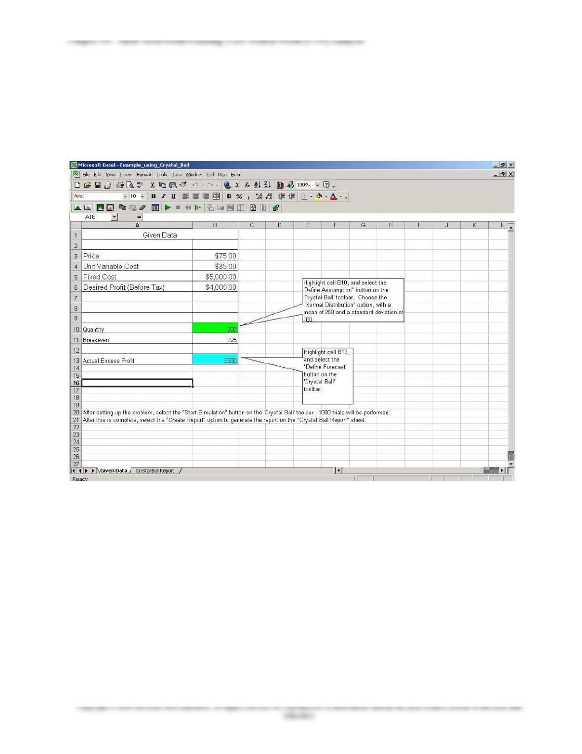
An example application in illustrated in Exhibit 1. Assume the information about price, unit variable cost,
fixed cost, desired profit, and expected sales quantity is given, as shown at the top of the spreadsheet. Any
one or more of these variables can be made into random variables within Crystal Ball. The only requirement
for Crystal Ball is that the numbers in the cells (B3: B6 and B10) must be numerical and NOT formulas.
Suppose the management accountant is uncertain about the sales quantity variable, which is now set at 300.
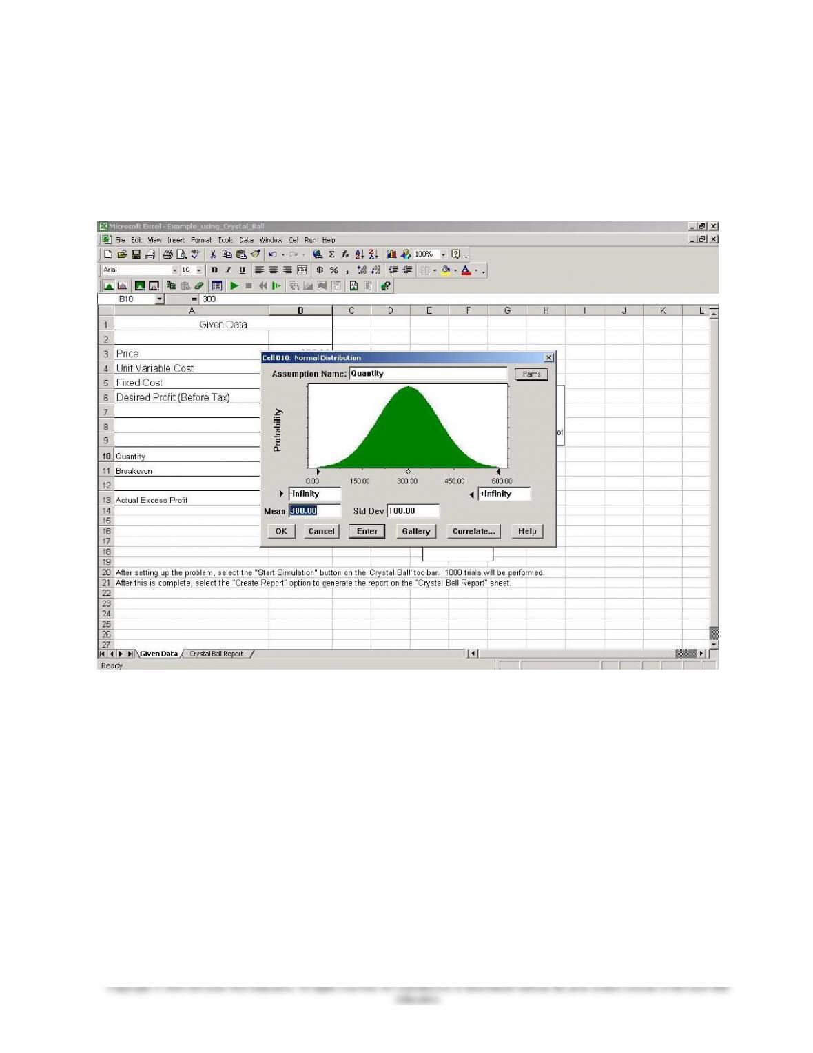
Crystal Ball allows you to select a probability distribution to represent your uncertainty about this variable.
See for example Exhibit 2, in which we have chosen a normal distribution for sales quantity with a mean of
300 and a standard deviation of 100 (other probability distributions are also available in Crystal Ball). The
selection is accomplished by choosing the “Assumptions” button on the command line, the one on the far left.
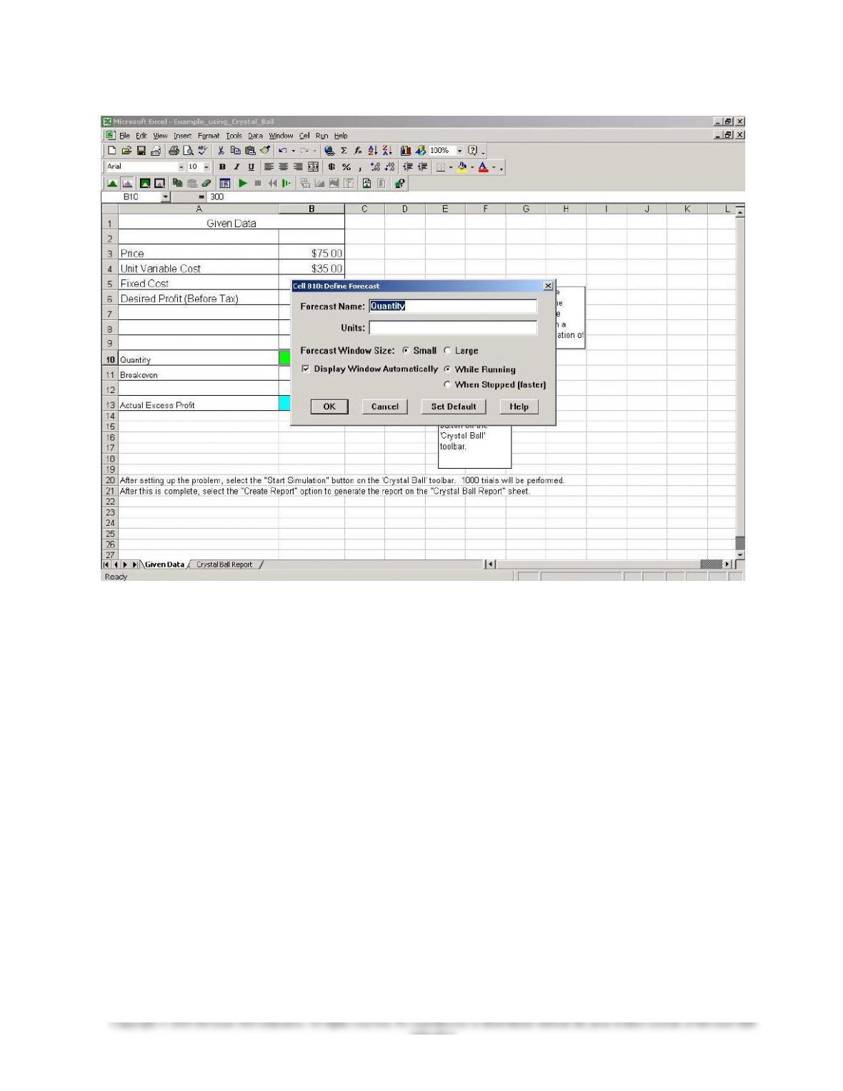
The next step is to choose a forecast (the simulated amount), which in this example is the amount of excess
profit (profit above the desired profit level), as determined from the formula in cell B13. The accountant
9-14
Chapter 09 - Short-Term Profit Planning: Cost-Volume-Profit (CVP) Analysis
wants to know the effect on this forecast amount of variations in sales quantity. To do this select the “Define
Forecast” button on the command line, the one next to the Assumptions button, that is, the one next to the left
side of the command line. The dialog box in Exhibit 3 will appear; it will show “quantity” as the variable
name and let you indicate the full name of the forecast variable (“units”) if you wish. Note also that the
contents of cell B13 must be a formula.
Exhibit 2: Determining a Probability Distribution within Crystal Ball
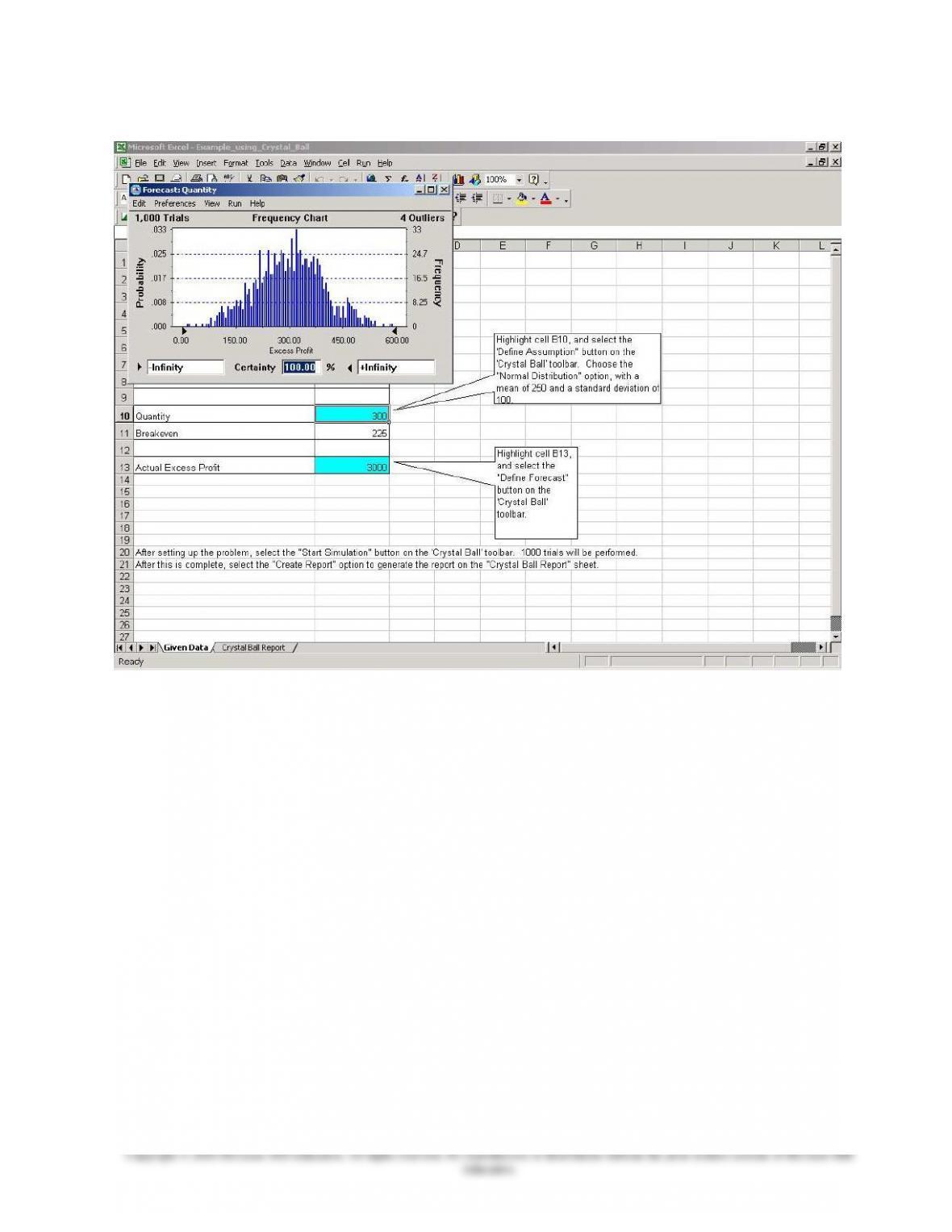
The final step is to run the simulation, which is done by selecting the right arrow button on the command line
(nine buttons from the left side). This will produce the simulation results shown in Exhibit 4. The frequency
chart shows the distribution of Excess Profit based upon the information entered in the spreadsheet and the
normal distribution selected for Quantity. To improve on the analysis the management accountant can select
additional variables to be probability distributions (two or more at a time is OK), and select alternative types
of distributions. Note that if you want to run another simulation you must first reset the program by choosing
the left pointing arrow on the command line. There are a variety of possible models and reports, up to the
discretion of the user.
9-15
Chapter 09 - Short-Term Profit Planning: Cost-Volume-Profit (CVP) Analysis
Exhibit 3: Selecting the Forecast in Crystal Ball
9-16
Education.
Chapter 09 - Short-Term Profit Planning: Cost-Volume-Profit (CVP) Analysis
Exhibit 4: Simulation Results in Crystal Ball
3. Non-linear Cost and Revenue Functions
This note expands the chapter presentation by showing the use of non-linear cost and revenue lines in CVP
analysis. Suppose the following cost and revenue behavior patterns have been observed for CAMPdeLUX, a
manufacturer of custom campers of the type which can be towed behind an auto or truck.
Total Revenues:
Total Costs:
These equations are such that there are three relevant ranges to the output of Q: (1) for low values of Q, total
costs exceed revenues, and (2) at higher values of Q revenues exceed total costs, and finally (3) at the highest
levels of Q total costs again exceed total revenues. Thus, the total cost and total revenue lines intersect at two
pointsa relatively low point (point A) and a high point (point C). The range of profit falls between these two
points, and the point of maximum profit (point B) is where the cost and revenue lines are parallel to each
9-17
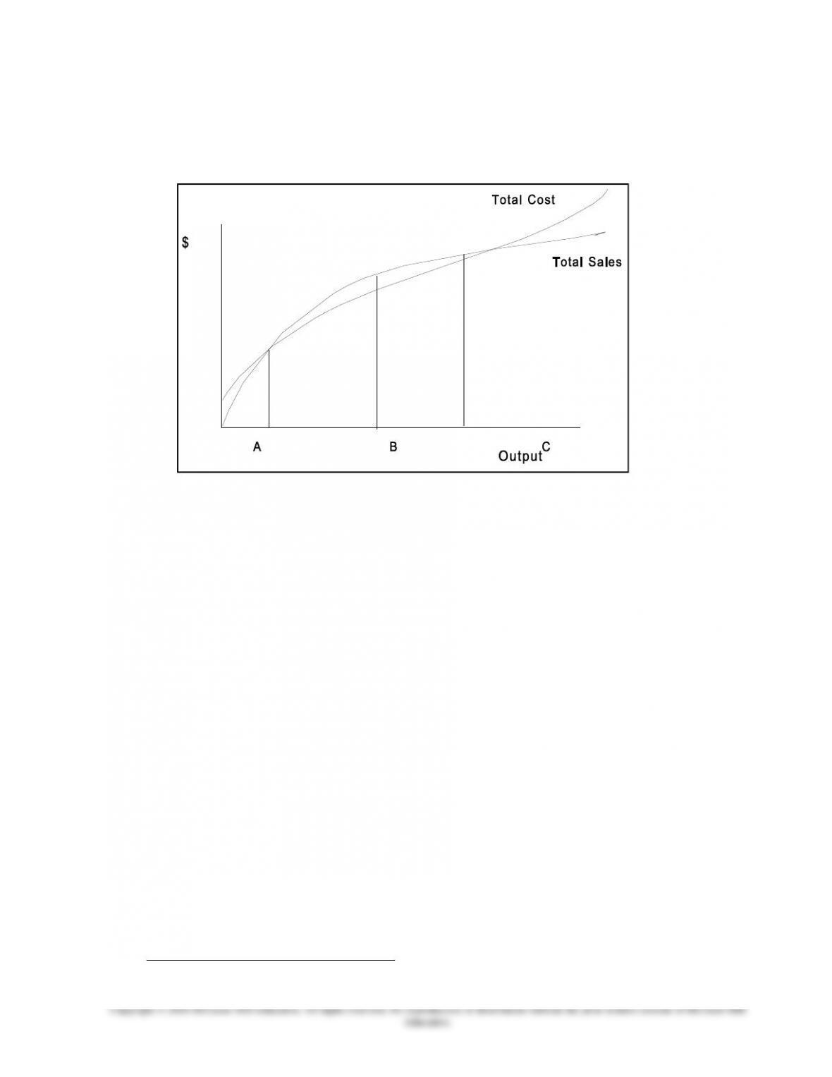
Chapter 09 - Short-Term Profit Planning: Cost-Volume-Profit (CVP) Analysis
other. Points A and C are the two breakeven quantities in this situation. These points can be found through the
solution of the cubic equation, which sets total revenue equal to total cost:
The solution of the above equation provides the two points, A = 3.2, and C = 41.6. Thus, we can see that
CAMPdeLUX will be profitable within the approximate range of 3 to 42 units, based upon present cost and
revenue characteristics.
To find the point of maximum profit (point B), we find marginal revenue (MR) and marginal cost (MC) for
CAMPdeLUX, and solve for the activity level where marginal revenue equals marginal cost, that is, the point
where the additional cost of one output equals the revenue for that particular item.
AND:
Q = +25 or −25
Since production must be positive, the point of maximum profit is 25 units. Thus, the use of differential
calculus allows us to develop concrete expectations for the range of profit and for the point of maximum
profit in those cases where the manager has good information on the curvilinear nature of costs and revenues.
Of course, variations on the above approach are possible where, for example, it is assumed that revenues are
linear while costs are curvilinear, or that costs are best described by a quadratic equation rather than a cubic,
and so on. Such variations can be adapted within the broad framework set out above.
4. Breakeven Determination Under Absorption Costing
Under Variable Costing (discussed in Chapter 18) there is a unique break-even point, independent of the
relationship between output volume and sales volume. Under variable costing, this same break-even point
would hold but only under a specific condition, i.e., only when the change in inventory is zero (that is, when
production = sales). In general, however, under absorption costing the break-even point depends on the
relationship between sales volume and production volume, as indicated by the equations below:
Break-even point under Variable Costing
9-18

Chapter 09 - Short-Term Profit Planning: Cost-Volume-Profit (CVP) Analysis
Q = F ÷ (p – v)
Break-even point under Absorption (Full) Costing
Q = (F + [Fixed overhead rate × (B/E unit sales – Output Volume)]) ÷ (p – v)
What the second equation shows is that, in general, under absorption costing the Breakeven quantity, Q, is
affected by the deferral (or drawing down of previously deferred) fixed overhead in inventory. Thus, under
absorption costing the break-even point is not easily determined. Rather, that breakeven point is a function of:
1. the level of projected fixed overhead costs
2. the denominator volume (activity level chosen for the predetermined overhead application rate)
3. the level of non-production-related fixed costs (such as marketing)
4. production volume
5. sales volume
6. the contribution margin per unit
7. how the company disposes of the production volume variance for the period
The preceding complications can be used to stress the advantage, for profit-planning purposes, of using a
variable costing approach to income determination. All of the formulas in Chapter 9 are developed and
presented under this assumption.
9-19
Education.


