
Chapter 09 – Short-Term Profit Planning: Cost-Volume-Profit (CVP) Analysis
Chapter 9
Short-Term Profit Planning: Cost-Volume-Profit (CVP) Analysis
Learning Objectives
LO 9-1 Explain cost-volume-profit (CVP) analysis, the CVP model, and the strategic role of CVP
analysis.
LO 9-2 Apply CVP analysis for breakeven planning.
LO 9-3 Apply CVP analysis for profit planning.
LO 9-4 Apply CVP for activity-based costing (ABC).
LO 9-5 Understand different approaches for dealing with risk and uncertainty in CVP analysis.
LO 9-6 Adapt CVP analysis for multiple products/services.
LO 9-7 Apply CVP analysis in not-for-profit organizations.
LO 9-8 Identify the assumptions and limitations of CVP analysis.
New in This Edition
Inclusion of a new reference (Zivney & Goebel, 2013) for expanding the basic CVP model to include
fixed financing costs and for deriving an alternative specification for Degree of Operating Leverage
(DOL), as Q ÷ (Q – B/E), where B/E equals the breakeven point defined in terms of volume, Q. See
T. Zivney and J. Goebel, “The Relationship between the Breakeven Point and Degrees of Leverage,”
Journal of Financial Education 11 (2013), pp. 122–126.
New discussion of using the Data Table option in Excel to present results of simple “What-If”
analyses
Newly added reference (McKee & McKee, 2014) for using Excel to perform basic Monte Carlo
Simulation (MCS) analysis (Thomas E. McKee and Linda J. B. McKee, “Using Excel to Perform
Monte Carlo Simulations, Strategic Finance, December 2014, pp. 47-51.)
Two updated Real-World Focus (RWF) items plus two entirely new RWF items (one dealing with
cost-structure analysis, the other dealing with operating leverage)
Six revised end-of-chapter problems
Graphical analysis of alternative cost-structure choice (including sensitivity analysis)
Increased use of Excel’s Goal Seek function throughout assignment material
Teaching Suggestions
I typically cover this chapter following Chapter 8. I explain that in Chapter 8 we show how costs behave and
how to develop cost-estimation models from actual data. These models are then used in Chapters 9, 10, 11,
and 12—to support managerial planning and decision-making. The cost-estimation models are used in
Chapter 9 directly, as a basis for understanding the relationships between costs, volume and profit—the CVP
model, which is couched as a short-term profit planning model in the sense that it captures the five factors
that, in the short run, combine to determine operating profits: sales volume, sales mix, variable cost per unit,
total fixed costs, and selling price per unit. I then explain that in Chapter 10 the cost-estimation models are
used to predict future costs in conjunction with the development of the master budget. Accurate prediction of
costs and revenues is critical to the master budgeting process. Chapter 11 deals with decision-making and cost
planning, and thus the ability to accurately predict costs and revenues is a key part of Chapter 11 as well.
Finally, in Chapter 12 we cover capital budgeting (i.e., long-term investment analysis). Inputs in capital
budgeting decision models generally include forecasted cost and cash flow data. In this way, I show the
following integrating themes for all five chapters (cost estimation, cost-volume-profit analysis, the master
budget, short-term decision-making, and capital budgeting):
9-1
Chapter 09 – Short-Term Profit Planning: Cost-Volume-Profit (CVP) Analysis
1) The key role of cost estimation in planning and decision making
2) The strategic importance of accurate cost estimates
I typically teach Chapter 9 in two class periods (this depends, however, on the level of prior exposure of the
students to the material in this chapter; in cases where the level of exposure is light-to-nonexistent, two
classes are probably needed to cover all aspects of the single-product/service case). In the first class (or first
two classes, as appropriate) I explain the basic model and then show the equation and contribution margin
methods for determining the breakeven point, both in terms of units and in terms of sales dollars. I explain
that the concept of breakeven is a broad one, and that it can be extended to include:
1) Targeted before tax profit, πB, or targeted after tax profit, πA (as such, the breakeven
point is simply a specific case of a more general model)
2) A long-term or a short-term perspective. I explain that in the long term all fixed costs
belong in the calculation; but in the short term, only incremental fixed costs are used.
3) Service, manufacturing, retail, and not-for-profit organizations (I try to show at least
one example of each)
In the second class period I cover multiple-product/service CVP (including a graphical analysis), operating
leverage, and the limitations of CVP. My major focus in the second day is on operating leverage, the degree of
operating leverage (DOL) as a measure of operating risk, and how DOL is used for a strategic analysis of the
firm. I make the point that high leverage can be associated with a more risky approach—one in which the firm
is more confident of the prospects for steadily increasing sales. At this point I have the class identify specific
firms that have high operating leverage and firms that have low operating leverage and we discuss the
strategic implications of the choice. Time permitting, I draw a parallel operating leverage and financial
leverage, noting in the process that the two can be measured and then combined to yield a total measure of
risk.
Assignment Matrix—Chapter 9
End-of-Chapter Exercises &
Problems Chapter Learning Objectives (LOs) Text Features
7th
ed.
6th
ed.
Transition
6e to 7e
X = included in Connect
Est.
Time
1. CVP analysis and strategy
2. Breakeven planning
3. Profit planning
4. ABC CVP analysis
5. Dealing with risk and uncertainty
6. CVP analysis for multiple products
7. Non-profit CVP use
8. Assumptions and limitations of CVP
Strategy
Service
International
Ethics
Sustainability
Brief Exercises
9-11 9-11 – X 5 min X
9-12 9-12 – X 5 min X
9-13 9-13 – X 5 min X
9-14 9-14 – X 5 min X
Continued on next page…
Chapter 9 Assignment Matrix—Continued
9-2
Education.
Chapter 09 – Short-Term Profit Planning: Cost-Volume-Profit (CVP) Analysis
7th
ed.
EOC
6th
ed.
EOC
Transition
6e to 7e
X = included in Connect
Est.
Time
1. CVP analysis and strategy
2. Breakeven planning
3. Profit planning
4. ABC CVP analysis
5. Dealing with risk and uncertainty
6. CVP analysis for multiple products
7. Non-profit CVP use
8. Assumptions and limitations of CVP
Strategy
Service
International
Ethics
Sustainability
9-15 9-15 – X 10 min X
9-16 9-16 – X 10 min X
9-17 9-17 – X 5 min X
9-18 9-18 – X 10 min X
9-19 9-19 – X 5 min X
9-20 9-20 – X 10 min X
Exercises
9-21 9-21 – X 25 min X X
9-22 9-25 – X 25 min X X
9-23 9-31 – – 30 min X
9-24 9-27 – – 25 min X X X
9-25 9-28 – X 20 min X X X X
9-26 9-23 Revised X 20 min X X
9-27 9-24 – X 15 min X X
9-28 9-29 – X 20 min X X X
9-29 9-22 – X 30 min X
9-30 9-26 X 20 min X X
9-31 9-35 X 20 min X X
9-32 9-36 – X 45 min X
9-33 9-30 – – 20 min X X X
9-34 9-34 Revised X 45 min X
9-35 9-33 Revised X 20 min X X X
9-36 9-32 – X 45 min X
Problems
9-37 9-37 Revised – 50 min X X X X
9-38 9-38 – – 60 min X X X X
9-39 9-39 Revised – 60 min X X X X
9-40 9-40 Revised – 50 min X X X
9-41 9-41 Revised – 30 min X X X
9-42 9-42 – – 60 min X X X X X
9-43 9-43 Revised – 50 min X X X X X
9-44 9-44 – – 75 min X X X
9-45 9-45 Revised – 60 min X X X X
9-46 9-46 – – 75 min. X X X X X
9-47 9-47 – – 45 min X X X
9-48 9-48 Revised – 90 min X X X X X X X
9-49 9-49 – – 90 min X X X X X X
9-50 9-50 – – 75 min X X X X X X
Lecture Notes
A. Cost-Volume-Profit (CVP) Analysis. Cost-volume-profit (CVP) analysis is a method for analyzing how
operating decisions and marketing decisions affect operating income based on the understanding of the
9-3

Chapter 09 – Short-Term Profit Planning: Cost-Volume-Profit (CVP) Analysis
relationship between variable costs, fixed costs (other than financing costs), unit selling price, output level
(sales volume), and sales mix. CVP analysis is based on an explicit model of the relationship between its three
factors (costs, revenues, and profits) and then they change in a predictable way as the volume of activity
changes. The basic (one-product or service) CVP model is:
πB = (p × Q) + (v × Q) − F
where: Q = units sold (i.e., volume)
v = unit variable cost
F = total fixed operating cost
p = unit selling price
πB = operating profit (pre-tax income, before unusual, extraordinary items, etc.)
Contribution Margin and Contribution Income Statement. The unit contribution margin is the difference
between unit sales price and unit variable cost:
p – v = Contribution margin per unit
The unit contribution margin measures the increase in profits for a unit increase in sales. The total
contribution margin is the unit contribution margin multiplied by the number of units sold. A measure of the
profit contributions per sales dollar is the contribution margin ratio, which is the ratio of the unit contribution
margin to unit sales price (p – v)/p. A useful way to show the information developed in CVP analysis is to use
the contribution income statement. The contribution income statement begins with revenues and subtracts
variable and fixed costs to obtain the total contribution margin and net income, respectively. The key
advantage of the contribution income statement is that it provides an easy and accurate prediction of the effect
of a change in sales on profits. This is not possible with the conventional income statement, which does not
separate variable and fixed costs.
B. Strategic Role of CVP Analysis. CVP analysis plays an important role in a firm’s strategic management.
In life-cycle costing, CVP analysis is used in the early stages of the product’s cost life-cycle to determine
whether the product is likely to achieve the desired profitability. Similarly, CVP analysis can assist target
costing at these early stages by showing the effect on profit of alternative product designs. In addition, CVP
analysis can be used at later phases of the life cycle to determine the most cost-effective manufacturing
process. CVP also has a role in strategic positioning. A firm that competes on cost leadership needs CVP
analysis primarily at the manufacturing stage, while a differentiating firm needs CVP analysis in the early
phases of the cost life cycle.
C. CVP Analysis for Breakeven Planning. The starting point in many business plans is to determine the
breakeven point, the point at which revenues equal total costs and profits are zero. This point can be
determined by CVP analysis. The CVP model is solved by inserting known values for, v, p, and F, setting πB =
equal to zero, and then solving for Q. There are multiple ways to solve for Q:
1. Equation Method: For Breakeven in Units. The equation method uses the CVP model directly.
2. Equation Method: For Breakeven in Dollars. Sometimes units sold, unit variable cost, and
sales price are not known. In this case, it is not practical to find the breakeven on units, but it is
possible to find the breakeven in sales dollars. We use the equation method in a revised form, where Y
is the breakeven point in sales dollars:
Y = [(v/p) × Y] + F
9-4

Chapter 09 – Short-Term Profit Planning: Cost-Volume-Profit (CVP) Analysis
This model is equivalent to the model used earlier for breakeven in units, except that Q is replaced by
Y/p, which produces the above equation (see text, p. 303).
3. Short-Cut Formulas. A convenient method for calculating the breakeven point is to use the
equation in its equivalent algebraic form (derived by solving the CVP breakeven model for Q):
Q = Fixed costs/Contribution margin per unit
= F ÷ (p – v)
The contribution margin method produces the same results as the equation method. The contribution
method can also be used to obtain breakeven in dollars, using the contribution margin ratio
(replacing p × Q with Y and solving for Y):
Y = (F + πB) ÷ ((p – v)/p)
Y = F ÷ ((p – v)/p)
Where: (p – v)/p = the contribution margin ratio
πB = 0 in this case (i.e., at breakeven, πB = 0)
4. CVP Graph and the Profit-Volume (PV) Graph. The CVP graph illustrates how the levels of
revenue and total costs change over different levels of output. The profit-volume (PV) graph
illustrates how the level of profits changes over different levels or output. The slope of the profit-
volume line is the unit contribution margin; therefore, the profit-volume graph can be used to read
directly how the total contribution margin, and therefore profits, change as the output level changes.
Both graphs are illustrated in text Exhibit 9.4.
D. CVP Analysis for Revenue and Cost Planning. CVP can be used to determine the level of sales needed
to achieve a desired level of profit.
1. Revenue Planning. CVP analysis assists managers in revenue planning to determine the revenue
required to achieve a desired level of profit. (See the equations presented in text p. 306.)
2. Cost Planning. For cost-planning decisions, the manager knows the value of Q and the desired
pre-tax profit, πB, but needs to find the value of the required variable cost per unit, v, or total fixed
cost, F. To facilitate target costing, CVP analysis is used to determine the most cost-efficient trade-
off between different types of costs. Another cost planning use of CVP analysis is to determine the
most cost-effective means to manage downstream costs, such as selling costs. Also, the manager’s
decisions about prices and costs usually must include income taxes because taxes affect the amount
of profits for a given level of sales. As indicated in text Exhibit 9.5, the Goal Seek function in Excel
can be used for cost (and revenue) planning using CVP analysis.
3. Extension of pre-tax profit planning, πB, to after-tax profit planning, πA, given a combined income
tax rate, t. First, express after-tax profit, πA, in terms of pre-tax dollar equivalents, πB, using the
following formula: πB = πA ÷ (1 – t). Second, use any of the preceding approaches for profit-planning
purposes (which approaches are based on targeted pre-tax profit, πB).
E. CVP Analysis for Activity-Based Costing. While the conventional approach to CVP analysis is to use a
volume-based measure, an alternative approach is activity-based costing (ABC). ABC identifies cost drivers
for detailed-level indirect cost activities. ABC provides a more accurate determination of costs because it
9-5

Chapter 09 – Short-Term Profit Planning: Cost-Volume-Profit (CVP) Analysis
separately identifies and traces indirect costs to products rather than combining them in a pool of fixed costs.
To use the activity-based CVP, first we define new terms for fixed cost: F = FVB + FAB,
where: FVB = the volume-based fixed costs, the portion of fixed costs that do not vary with the activity-
based cost driver
FAB = the portion of fixed costs that do vary with the activity-based cost driver
Second, we define the following terms:
vAB = the cost per batch for the activity-based cost driver
b = the number of units in a batch
vAB/b = the cost per until of product for batch-related costs when the batch is size b
Third, the CVP model for ABC is:
Q = (FVB + πB) ÷ (p – v – (vAB ÷ b))
This method assumes that we hold batch size constant and vary the number of batches as the total volume
changes. CVP analysis based on ABC can provide a more precise analysis of the relationships among
volume, cost, and profits by considering batch-level costs.
F. Dealing with Risk and Uncertainty. Sensitivity analysis is the name for a variety of methods that
examine how an amount changes if factors involved in predicting that amount change. Sensitivity analysis is
particularly important when a great deal of uncertainty exists about the potential level of future sales volumes,
prices, or costs. We discuss the following methods for dealing with risk and uncertainty in short-term profit
planning:
1. What-if Analysis of Sales: Contribution Margin and Contribution Margin Ratio. What-if
analysis is the calculation of an amount given different levels for a factor that influences that
amount. Many times it is based on the contribution margin and the contribution margin ratio.
2. Decision Tables/Decision Trees/Expected Value Analysis
3. Monte Carlo Simulation (MCS)
Other Measures of Risk:
1. Margin of Safety. The margin of safety measures the potential effect of a change in sales on
profits:
Margin of safety = Planned (or actual) sales – Breakeven sales
“Sales” in the preceding formula can be defined either in terms of dollars or in terms of units.
The margin of safety (MOS) also can be used as a ratio, a percentage of sales:
Margin of safety ratio (MOS%) = Margin of safety (MOS) ÷ Planned (or actual) sales
MOS% is a useful measure for comparing the risk of two alternative products or for assessing the
risk in any given product. The product with a relatively low margin of safety ratio is the riskier of
the two products and therefore usually requires more or management’s attention.
9-6
Education.

2. Operating Leverage. This refers to the mix of variable versus fixed costs in an organization’s
cost structure. The potential effect of the risk that sales will fall short of planned levels is
measured by the following “sensitivity” ratio, called degree of operating leverage (DOL):
DOL = Contribution margin ÷ Operating income
DOL is calculated and interpreted at each volume level, Q. DOL will be a percentage equal in
amount to the percentage change in operating income for each percentage change in sales (up or
down), from the specified sales volume level, Q.
A higher value for DOL indicates a higher risk in the sense that that a given change in sales will
have a relatively greater impact on profits. (Put another way, a higher DOL implies greater
sensitivity of changes in operating income—both up and down—in response to changes in sales
volume.) When sales volume is strong, a high level of leverage is desirable, but when sales begin
to fall, a lower level of leverage is preferable.
The instructor can draw a parallel here to the notion of financial leverage, which relates to the
relative mix of debt vs. equity in a firm’s capital structure. The higher the ratio of debt to equity
(i.e., the greater the financial leverage), the higher the risk (traceable to the existence of higher
levels of fixed interest payments).
G. CVP Analysis with Multiple Products (or Services). Given an additional assumption, it is possible to
use CVP analysis for multiple products (or services). Our adaptation on the CVP model requires one key
assumption: the sale of the products will continue at a prescribed sales mix. That is, the sales of each product
will remain at the same proportion of total sales. The mix can be determined in either sales units or sales
dollars (but the mix percentages will generally differ between these two approaches). Assuming a constant
sales mix allows us to treat the two or more products as one combined product mix by computing a weighted-
average contribution margin (either per unit or ratio). The weighted-average contribution margin is used to
determine the total sales necessary to attain the desired operating result.
H. CVP Analysis for Not-for-Profit (NFP) Organizations. Not-for-profit organizations can also use CVP
analysis; examples include determining the drop in capacity due to a budget cut, or using CVP analysis to
identify profitable new services and to help analyze the cost of delivering existing services.
I. Assumptions and Limitations of CVP Analysis.
1. Linearity, the Relevant Range, and Step Costs. The CVP model assumes that revenues and
total costs are linear over the relevant range of activity. The caution for the manager is therefore
to remember that the calculations performed within the context of a given CVP model should not
be used outside the relevant range.
Step costs. Sometimes the cost behavior under examination may be so “lumpy” (step costs) that
an approximation via a relevant range is unworkable. Although CVP analysis can still be done, it
becomes somewhat more cumbersome.
2. Identifying Fixed and Variable Cost for CVP Analysis. In CVP analysis, it is not always easy to
determine the dollar figures used for fixed costs and unit variable costs.
a. Fixed costs to include. In a short-term analysis, relevant fixed costs are those expected to
change with the introduction of the new product. In contrast, for a long-term analysis of
9-7

Chapter 09 – Short-Term Profit Planning: Cost-Volume-Profit (CVP) Analysis
breakeven, all current and expected future fixed costs associated with the production,
distribution, and sale of the product are relevant.
b. The period in which the cost was incurred. The fixed costs in a CVP analysis can include the
expected cash outflows for fixed costs in the period for which breakeven is expected;
alternatively, they can include the fixed costs as determined by accrual accounting. The
advantage of the cash flow approach is its focus on the company’s cash needs. However, the
advantage of the accrual method is that is ties the CVP analysis to the income statement.
c. Unit variable costs. In measuring unit variable cost, the management accountant must be
careful to include all relevant variable costs, not only for production costs, but also selling and
distribution costs.
The Five Steps of Strategic Decision Making for CVP Analysis
Here is an example to illustrate strategic decision making in CVP analysis. Russ Talmadge operates a real
estate service business that provides rental management services, real estate appraisal, and a variety of other
services. Russ is successful because of his knowledge and experience and the reliability of his service which
has gained him the trust of his customers, many of whom have been with him for several years. One of the
key items in his office is a printer that prints copies of photos from his digital camera. The photos are used in
appraisals and in other services. His copier was relatively inexpensive to buy ($99) but the ink cartridges are
expensive—depending on the capacity of the cartridge, the cost is from $37.50 for a capacity of 500 copies to
$80 for a capacity for 2,000 copies. Russ prints about 1,000 photos a month.
1. Determine the Strategic Issues Surrounding the Problem. Russ’s business is based on his knowledge
and reliable service. The photos that are a part of his service must also be produced reliably (no printer jams
or delays getting the photo to the customer) and of high print quality.
2. Identify the Alternative Actions:
Russ can purchase the high capacity cartridge (2,000 copies) or the low capacity cartridge (500 copies) for his
printer. The high capacity cartridge will cost 4 cents per copy ($80/2,000) while the low capacity cartridge
will cost 7.5 cents per copy ($37.50 ÷ 500). Another option is to buy a new printer for $150 which has a
cartridge which costs $60 (capacity of 2,000 copies; 3 cents per copy).
3. Obtain Information and Conduct Analyses of the Alternatives
Option One: Retain current copier: The high capacity cartridge will cost $40 per month (1,000 copies
at 4 cents per copy) and the lower capacity cartridge which will cost $75 per month (1,000 copies at
7.5 cents per copy). The purchase cost of the copier can be ignored since it is a sunk cost, and
therefore the high-capacity cartridge will always be the low cost option.
Option Two: New Copier: The breakeven point for the new copier (assuming Russ is using the high
capacity cartridge on his current copier) would be 15,000 copies — $150 ÷ (4 cents – 3 cents) – or, 15
months of usage.
4. Based on Strategy and Analysis, Choose and Implement the Desired Alternative
Option One: The choice of cartridge has no effect on the quality or reliability of the printer, so the
choice can be made on the basis of lower cost, and in this case the high capacity cartridge is preferred.
9-8

Chapter 09 – Short-Term Profit Planning: Cost-Volume-Profit (CVP) Analysis
Also, the high-capacity cartridge would mean less frequent cartridge replacement, and therefore less
chance of a potential delay when a photo is needed quickly.
Option Two: Russ would get breakeven on the new copier in 15 months, not a particularly long period
given the number of years he has been in business. And the addition of a new copier would give him
a “backup” if one of them should fail. However, looking at a Consumer Reports study of copiers,
Russ finds that the $150 copier does not have as high a reliability or quality rating as does his current
copier. Considering the importance of quality and reliability in his business, Russ chooses option one
with the high capacity cartridge.
5. Provide an On-going Evaluation of the Effectiveness of implementation in Step 4.
Russ continues to review the available printers. If he determines a way to reduce the need for photos, or can
print them on a color printer instead of photo paper, he may be able to reduce costs substantially. He may also
be able to obtain the cartridges at lower cost from a new supplier.
Advanced Lecture Notes
There are four advanced lecture notes for Chapter 9:
(1) A graphical analysis for CVP with two products
(2) Additional topics in sensitivity analysis (analytical methods, simulation methods)
(3) The case of non-linear cost and revenue, and
(4) Break-even under absorption costing
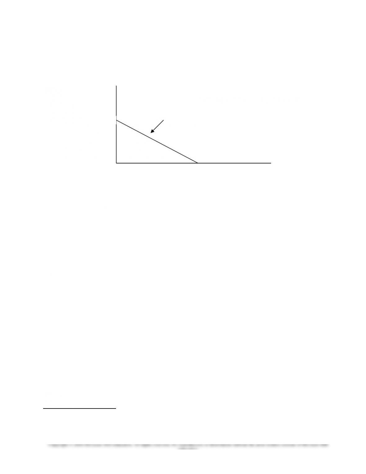
1. A Graphical Analysis for CVP with Two Products
When only two products are involved, a graphical approach can add to the manager’s understanding of the
cost-volume relationships for these products. The analysis is based on the fact that the breakeven point for the
firm can be any one of many possible combinations of sales mixes for the two products. Fortunately, all
possible combinations of sales mixes for breakeven are easy to identify graphically, once we know the
breakeven points of each product. Suppose only Windy and Gale (from the example in the text, Exhibit 9-9)
are produced, with individual breakeven points as follows:
Windy: $168,000 ÷ 8 = 21,000 units
Gale: $168,000 ÷ 4 = 42,000 units
All possible combinations of breakeven points lie on (and only on) the line joining the individual breakeven
points for the two products, as illustrated in the graph below. This is so because of the linear nature of the
CVP relationship for each of these products. Any point on the line can be determined from the equation for
that line, which is:
Units of Gale = (42,000 ÷ 21,000) × (21,000 – Units of Windy)
OR:
Units of Gale = 42,000 – (2 × #Units of Windy)
For example, the breakeven quantity for units of Gale, if Windy is sold at the level of 19,000 units, would be:
Units of Gale = 42,000 – (2 × 19,000) = 4,000 units of Gale
The total contribution margin of this particular product mix would be:
9-9
Education.
Chapter 09 – Short-Term Profit Planning: Cost-Volume-Profit (CVP) Analysis
(19,000 × $8) + (4,000 × $4) = $168,000
The graphical analysis can help the manager see that breakeven for two products can be achieved by many
different possible combinations of product mixes, specifically, all those product mix combinations that fall on
the line segment shown in the graph below.
2. Additional Topics in Sensitivity Analysis
Analytical Methods
When possible, an effective approach for sensitivity analysis is to use an analytical technique to derive a
model for the sensitivity of the breakeven point or profit to any of the cost factors in the CVP model. For
example, it can be shown algebraically or through differential calculus that the change in the breakeven point
is related to the change in fixed costs by the “sensitivity” factor, 1 ÷ (p − v).1 That is, as fixed costs change,
the breakeven point will change by the amount of the change in fixed cost times 1 ÷ (p − v). For example, if
price is $10, unit variable cost is $5, and fixed cost is $10,000, then the breakeven point is:
Q = $10,000 ÷ ($10 − $5)/unit = 2,000 units
And the sensitivity factor is:
1 ÷ (p − v) = 1 ÷ ($10 − $ 5) = 0.2
For example, if fixed costs increase by $5,000 from $10,000 to $15,000, then the breakeven point should
increase by 0.2 × 5,000 = 1,000 units.
The analytical approach can be used to determine the sensitivity of the breakeven point to changes in any of
the factors of the CVP model. The approach is most useful, however, when the question involves only a
couple of factors (as above, the manager wants to know the effect of a change in fixed costs on the change in
the breakeven level in units), and the decision requires mathematical precision. The analytical approach also
has the advantage of often providing a simple decision rule for assessing the sensitivity of one factor to
another, as in the above illustration relating fixed costs and the breakeven point.
1 See Horace R. Givens, “An Application of Curvilinear Breakeven Analysis,’ The Accounting Review (January 1966, pp.
141-143) for an illustration of the use of differential calculus in the CVP context.
9-10
Education.
Units of Windy
Any point on this line is a breakeven point
21,000
42,000 Units of Gale