Chapter 9 – Short-Term Profit Planning: Cost-Volume-Profit Analysis
As before, πB = TR – VC – FC
= (sp*X) – (vc*X) – FC = $5X
For Alternative #2:
πB = 0.05($60X) ÷ (1 – 0.40) = $5X
As before, πB = TR – VC – FC
= (sp*X) – (vc*X) – FC = $5X
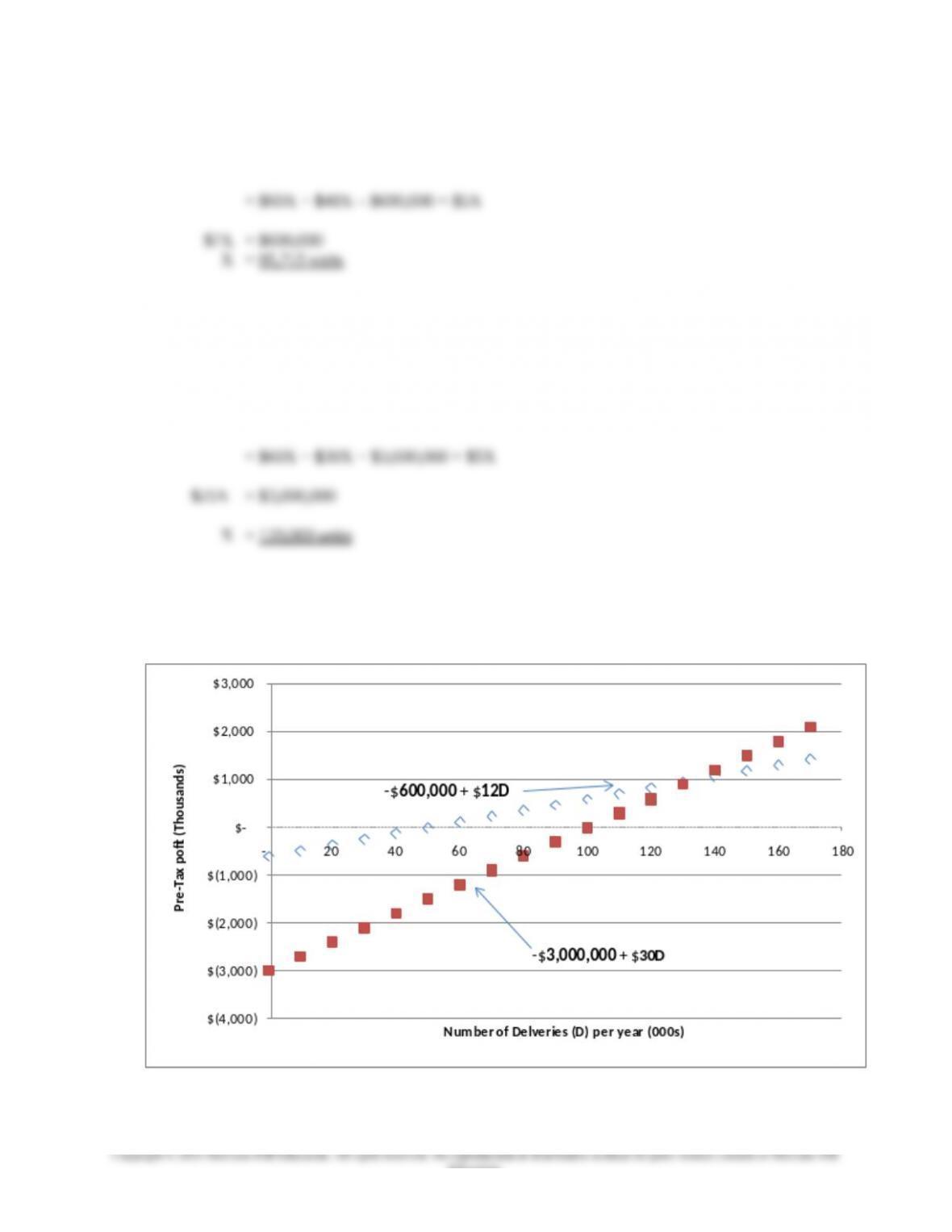
(9) Consider the original data in the problem. Construct a graph for each of the two alternatives
depicting pre-tax profit, πB, as function of volume (number of deliveries per year). Clearly label
the profit equation for each alternative.
9-18
Education.
Chapter 9 – Short-Term Profit Planning: Cost-Volume-Profit Analysis
(10) Based on the graphs prepared in (9), which decision-alternative do you think is the more
profitable one for this business?
We cannot say which firm’s cost structure is more profitable because, as indicated by a general CVP
graph, the level of pre-tax profit depends crucially on the level of sales volume. We can determine
that the indifference point is approximately 133,333 units per year. At this volume, the two cost
(11) Based on the original data and the graphs prepared above in (10), which decision alternative is
more risky to the business? Explain. (Hint: Think about, and define in your answer, the notion
of “operating leverage.”)
The contribution margin generated from sales must be sufficient to cover the fixed costs; any excess
after coverage of fixed costs translates directly into pre-tax profit. If the contribution margin is not
sufficient to cover the fixed costs, then a loss occurs for the period. That is, cost structures with
relatively higher amounts of fixed costs are riskier, just as firms with relatively high levels of debt in
their capital structure are more risky. A measure of the former is the “degree of operating leverage,”
while a measure of the latter is “financial leverage.” In other words, the degree of operating leverage
provides a measure of the risk-return trade-off that exists across different cost structures, such as the
two illustrated in this problem.
The degree of operating leverage is calculated at a given volume (output) level and is defined as:
Contribution Margin/Operating Income. The higher the degree of operating leverage, the greater the
changes in pre-tax profit—in both directions.
Note, however, that once the breakeven point has been reached, pre-tax profit increases by the
product of the unit contribution margin and the number of units sold. Thus, as seen from the above
graph, if volume is predicted to be high, the preferred cost structure is Alternative #2. Once the break-
even point is reached, a large portion of each sales dollar goes directly to operating income.
(12) Finally, in building your profit-planning (i.e., CVP) model, the analyst makes a number of
important assumptions. List the primary assumptions that underlie a conventional CVP
analysis, such as the ones you conducted above.
Any model is only as good (accurate) as the validity of the underlying assumptions of the model. The
following are the assumptions behind a traditional CVP model:
1. Revenues and costs (variable and total) change only in response to a single driver:
volume of sales. In fact, the term CVP derives precisely from this assumption.
9-19
2. Input variables (selling price per unit, variable cost per unit, total fixed costs, and for the
9-20
Education.

Chapter 9 – Short-Term Profit Planning: Cost-Volume-Profit Analysis
Case 9-7: Pancake World
Note to Instructor: The Pancake World Case is based on the actual experience and disguised data of a
franchise owner of one of the well-known pancake restaurants.
1) From the information that the annual number of guests, it is possible to get the average variable
cost per guest of $3.82 = $497,000 ÷ 130,000. Since the average ticket price per guest is $7.45,
breakeven in number of guests can be calculated as follows.
Fixed Costs ÷ (Selling Price − Variable cost) = number to break even
$281,000 ÷ ($7.45 − $3.82)/guest = 76,987 guests per year
76,987 guests per year ÷ 365 days per year = 211 guests per day.
Louis looks to the weekly managers’ report (Exhibit 3 under the guest count row near the bottom
of the Exhibit) to find out what the average guest count is for weekdays and the weekend.
Weekdays are Monday to Thursday and weekend days are Friday to Sunday. Average weekday
guest count is 415 guests. This shows a difference of 204 guests from the breakeven number.
Weekend average guest count is 633 guests. The difference is 422 guests from the breakeven
guest count. Louis sees a good safety margin.
Weekends tend to be busier than weekdays. Also, when holidays fall on a weekday this brings up
guest count and expenses. The annual breakeven gives a useful figure for planning. While
demand varies during the week, variable costs (food and labor) follow the demand, and fixed
costs tend to be monthly and/or annual. So, seasonality plays a minor role in breakeven analysis
over the course of a year.
2) Referring to Exhibit 3 under the Labor % row gives labor % breakdown per day. Calculating the
average for the week a figure of 22.5% labor cost has been achieved. This is one percentage point
below the company’s requirement. Labor cost is a significant part of operational expense and
keeping this figure along with total food cost % in line ensures profitability.
3) The use of CVP in Louis’s restaurant is critical. The profit margin average in the restaurant
industry is 10%. With strong competition being common for restaurants of this type, competing
on a good value makes it important to be cost-effective in all phases of operations, especially the
management of labor and food.
PW is a mature firm in a mature market. With low profit margins common in the industry, high
leverage could be an advantage, and it is often utilized in the industry through such techniques as
growth in number of restaurants and extending the number of hours the restaurant is open. On
the other hand, a key feature of the cost structure of the restaurant is that most costs are variable,
food and labor, so that it is difficult to achieve a high degree of operating leverage. One thing
that helps is to outsource some types of labor (e.g., payroll processing) and outsource some
aspects of food inventory (food delivery, by U.S. Foodservice Inc.) to allow the restaurant to
focus on customer service and improving customer loyalty.
9-21
Education.

Chapter 9 – Short-Term Profit Planning: Cost-Volume-Profit Analysis
Teaching Strategy for Readings
Reading 09-01: “Tools for Dealing with Uncertainty”
This article explains how to use simulation methods within a spreadsheet program such as Excel to
perform sensitivity analysis for a given decision context. The available spreadsheet simulation software
systems include the programs Crystal Ball and @Risk, among others. These software systems allow the
user to analyze the effect of uncertainty on the potential outcomes of a decision. These tools can be
applied directly to CVP analysis. The tools allow the user to see the potential effect on the breakeven
level or total profit of potential variations in the key uncertain factors in the analysis. The uncertain
factors affecting breakeven might be the unknown level of unit variable cost, price or fixed cost. Also, in
determining total profit, the unknown level of demand might be a key uncertain factor.
Exercise: Use a spreadsheet simulation tool such as Crystal Ball or @Risk to analyze the uncertain
factors in given case situation. Cases 9-1, 2 and 3 could be used or a problem from the text, for example,
Text problem 9-53, the Computer Graphics Case. This is illustrated in the “Advanced Lecture Notes”
section of the Instructor’s Resource Guide for Chapter 9.
9-22
Education.
Chapter 9 – Short-Term Profit Planning: Cost-Volume-Profit Analysis
Reading 09-2: Turning Budgets into Business—Part I of III
Introductory Note: This assignment assumes familiarity with the comprehensive master budget exercise
developed by Porter and Stephanson (see Strategic Finance, February–July, 2010). The Excel solution file
containing this master budget, and obtained from by the authors from Porter and Stephanson, is inserted
as an object below:
Bob‘s Bicycles –
Master Budget.xlsx
In addition, the following pdf file (which contains data and assumptions needed to construct the master
budget for Bob’s Bicycle) can be distributed to students in advance of covering the requirements of
Reading 09-02:
The purpose of Reading 09-02 is to have students use the Master Budget (which was highlighted in the
set of Budgets by Porter &Stephanson that were published in Strategic Finance during 2010—see
1. Add a Contribution Margin Income Statement to the aforementioned Master Budget.
2. Using the fixed-and variable cost information provided by this Income Statement, we’ll calculate the
breakeven point and margin of safety and discuss how these two important numbers can be used in
Student Lecture
Handout (Master Budg