Chapter 9 – Short-Term Profit Planning: Cost-Volume-Profit Analysis
TN-1: Example of Spreadsheet Solution for Alltel Case
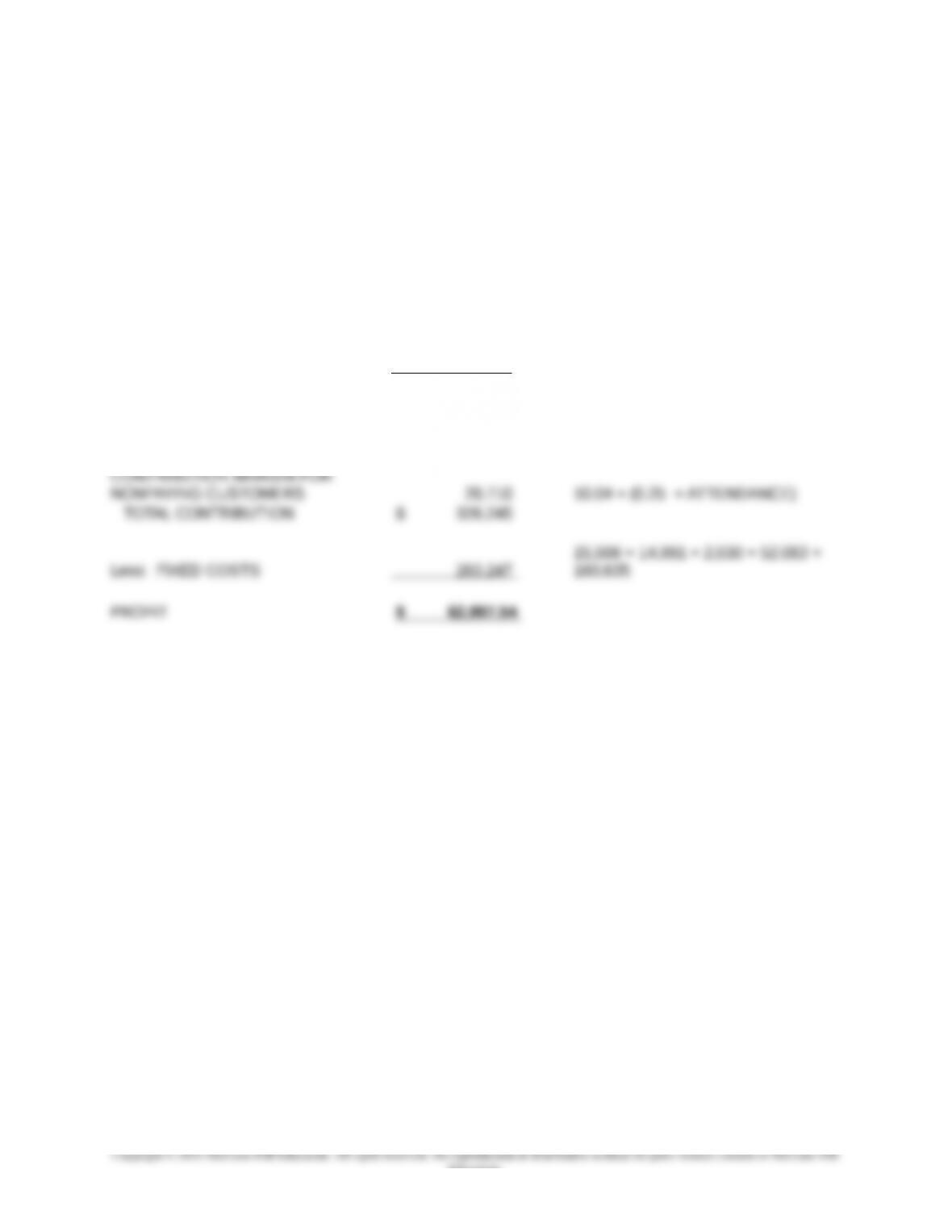
Alltel Pavilion
EXPECTED PAYING ATTENDANCE 8,251 GIVEN
TOTAL REVENUE FROM TICKETING
PER CAPITA $ 26.99 GIVEN
TOTAL REVENUE FROM
ANCILLARIES PER CAPITA $ 13.09 GIVEN
LESS 10% OF REVENUE 1.31 13.09 × 0.1
LESS VARIABLE EXPENSES 1.74 0.17 + 0.35 + 1.1.2 + 0.08 + 0.02
CONTRIBUTION FROM ANCILLARIES
PER CAPITA $ 10.04 13.09 − (13.09 × 0.10) − 1.74
CONTRIBUTION MARGIN FOR
PAYING CUSTOMERS 305,535 (26.99 + 10.04) × ATTENDANCE
9-11
Education.
Chapter 9 – Short-Term Profit Planning: Cost-Volume-Profit Analysis
Case 9-5: Sensitivity Analysis: Regression Analysis
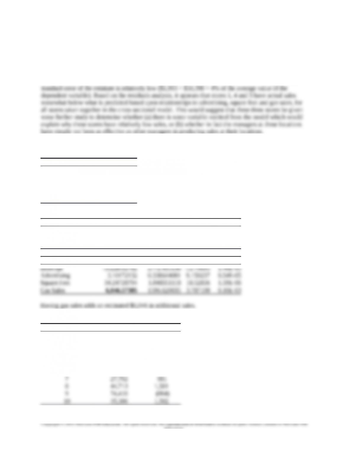
1. The regression analysis to identify the stores that seem to be operating at below their potential, based
on relationships for all the stores can be determined from a cross-sectional regression. The results are
shown below. Note that the regression has excellent measures for both reliability and precision. The t
values of each of the independent variables is significant (p < .05), the R-squared value is high and the
Note also that whether or not a store sell gasoline has a significant effect on total sales. For this data it
appears that gasoline contributes approximately $6,406 to total sales for locations selling gasoline.
Regression Statistics
Multiple R 0.997584458
R Square 0.995174751
Adjusted R Square 0.992762127
Standard Error 1993.16876
Observations 10
ANOVA
df SS MS F
Regression 3 4916081167 1.64E+09 412.48641
Residual 6 23836330.24 3972722
Total 9 4939917497
Coefficients Standard Error t Stat P-value
RESIDUAL OUTPUT
Observation Predicted Sales Residuals
1 57,299 (1,265)
2 22,181 864
3 88,073 1,264
4 68,005 (1,932)
5 21,970 (2,977)
6 64,160 766
9-12
Education.
Chapter 9 – Short-Term Profit Planning: Cost-Volume-Profit Analysis
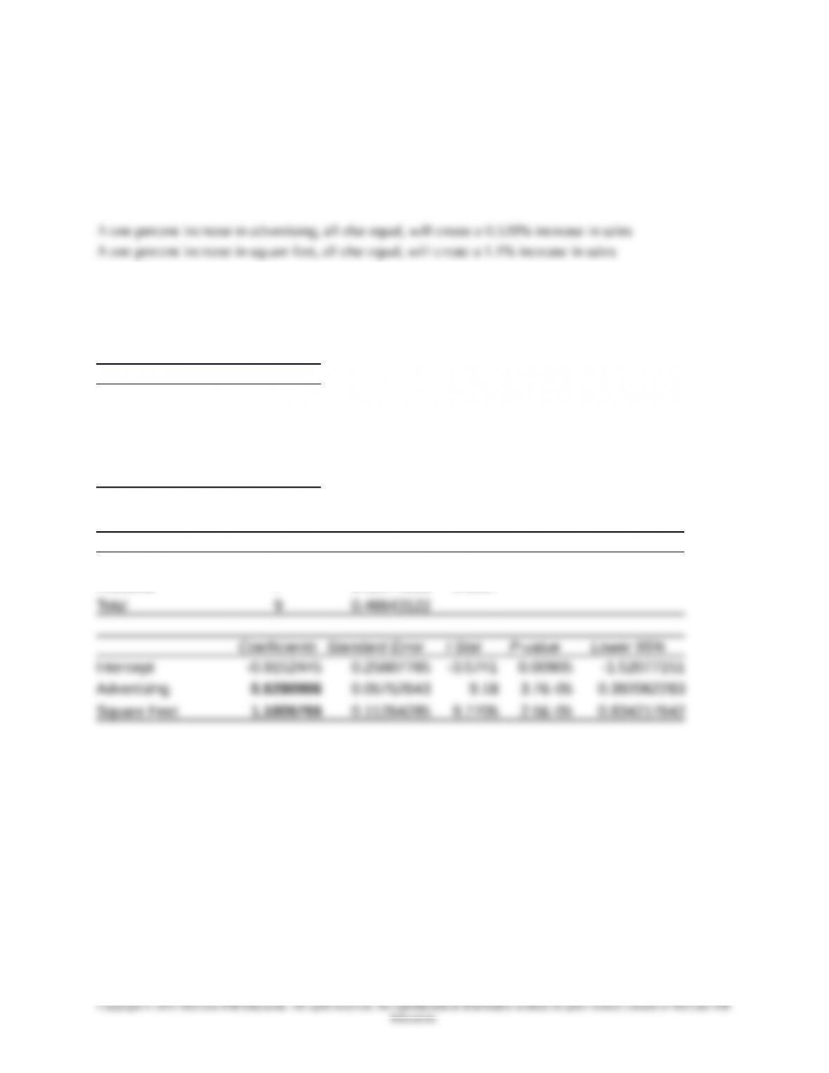
2. The analysis of the sensitivity of total sales to store size (square feet) and advertising can be
determined by taking the log transform for each of the data points and recalculating the regression. Note
again that the statistical measures for the regression are all excellent. Using the coefficients of the
independent variables, we can now find that:
This is useful information for Fast Shop in planning desired levels of advertising and for considering the
appropriate size for new locations and/or extensions to current locations.
Regression with Log Transforms on All Variables, except the Gas Sales (0,1) Variable
Regression Statistics
Multiple R 0.9948958
R Square 0.9898177
Adjusted R Square 0.9869084
Standard Error 0.0260476
Observations 10
ANOVA
df SS MS F Significance F
Regression 2 0.46168187 0.2308 340.233 1.06528E-07
Residual 7 0.00474936 0.0007
9-13
Chapter 9 – Short-Term Profit Planning: Cost-Volume-Profit Analysis
Case 9-6: Profit Planning—Choice of Cost Structure
Note to Instructor:
For those students seeking to become a Certified Management Accountant (CMA), the topic of CVP
analysis is an important one covered on the CMA exam. 1 In terms of this topic, the successful candidate
is expected to be able to:
demonstrate an understanding of how cost/volume/profit (CVP) analysis is used to examine
the behavior of total revenues, total costs, and operating income as changes occur in output
levels, selling prices, variable costs per unit, or fixed costs
differentiate between costs that are fixed and costs that are variable with respect to levels of
output
demonstrate an understanding of the behavior of total revenues and total costs in relation to
output within a relevant range
explain why the classification of fixed vs. variable costs is affected by the timeframe being
considered
demonstrate an understanding of how contribution margin per unit is used in CVP analysis
calculate contribution margin per unit and total contribution margin
calculate the breakeven point in units and dollar sales to achieve targeted operating income or
targeted net income
demonstrate an understanding of how changes in unit sales mix affect operating income in
multiple-product situations
demonstrate an understanding of why there is no unique break-even point in multiple-product
situations
analyze and recommend a course of action using CVP analysis
demonstrate an understanding of the impact of income taxes on CVP analysis
Recommended Solutions
(1) What is meant by the term “short-term profit-planning” model, and how can such a model be
used by management? (That is, in what sense can this model be used to facilitate planning,
control, or decision-making by managers of an organization?)
Short term operating profit can be modeled as a function of five factors: (1) selling price per unit; (2)
variable cost per unit; (3) total (short-term) fixed costs; (4) sales volume; and, (5) sales mix. A short-
term profit planning model combines these factors into a predictive model, that is, a model that can be
What volume of sales (in units or dollars) is needed to break even?
What volume of sales (in units or dollars) is needed to achieve a particular level of profit,
either on a pre-tax or post-tax basis?
1 Ceriied Management Accountant Learning Outcome Statements (efecive 7/1/04) (Updated 07-2008), available
at htp://www.imanet.org.tw/img/CMALOS.pdf.
9-14
What effect would a change in selling price per unit have on operating profit of all other
factors were held constant?
It is worthwhile to reduce sales price per unit in exchange for an estimated increase in
volume?
Which type of cost structure, one that has relatively high variable costs versus one that has
relatively high fixed costs, is preferable for an organization?
What is the percentage change in the break-even point for a given percentage change in fixed
costs?
At what volume level would the firm be indifferent between two alternative cost structures?
What would be the impact on the break-even point if all factors remained the same except
variable costs per unit decreased by a given number of dollars or a given percent?
From a risk perspective: how will projected operating profit be affected if volume is less than
predicted (e.g., 5% less, or 10% less)?
What is the “margin of safety” (in dollars, units, or percentage) for the coming accounting
period?
What is the likely effect on operating profits of a shift in sales (or service) mix?
Note that the organization’s CVP model can be depicted in equation form or in graphical form, of
which there are two alternative formulations: a cost-volume-profit graph, and a profit-volume graph.
(2) What is the definition of “fixed cost,” “variable cost,” “contribution margin ratio,”
“contribution margin per unit,” and “relevant range”?
The terms “fixed cost” and “variable cost” represent descriptions of cost behavior, that is, to
descriptions of how a given cost changes or reacts to changes in one or more cost drivers (activity
variables). A fixed cost, within an assumed range of activity or output, does not change in total as
activity changes. As such, we can say that a fixed cost is independent of changes in activity or output.
By contrast, a variable cost is one that changes in total as output or activity changes. On a per-unit-of-
activity basis, variable costs are said to be fixed. Implied in the process of classifying costs by
behavior is an assumed planning horizon or time period. Thus, the longer the time period, the greater
(3) What is the break-even point, in terms of number of deliveries per year (or per month), for
Alternative #1? For Alternative #2?
The break-even volume (X) (in this case # of deliveries) is given as:
9-15
Education.
Chapter 9 – Short-Term Profit Planning: Cost-Volume-Profit Analysis
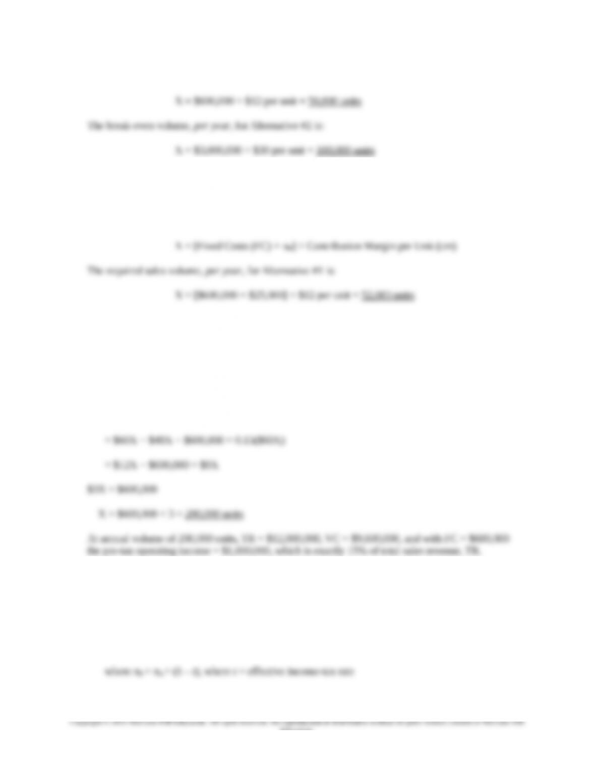
The break-even volume, per year, for Alternative #1 is:
(4) How many deliveries would have to be made under Alternative #1 to generate a pre-tax profit,
πB, of $25,000 per year?
The required sales volume (X) (in this case # of deliveries) is given as:
(5) How many deliveries (per year) would have to be made under Alternative #1 to generate a pre-
tax profit, πB, equal to 15% of sales revenue?
We begin with the following general profit equation, where X = sales volume:
πB = TR – VC – FC
= (sp*X) – (vc*X) – FC = 0.15 (sp*X)
(6) How many deliveries would have to be made under Alternative #2 to generate an after-tax
profit, πA, of $100,0000 per year, assuming a tax rate of, say, 45%?
The required sales volume (X) (in this case # of deliveries) is given as:
X = [Fixed Costs (FC) + πB] ÷ Contribution Margin per Unit (cm)
9-16
Education.
Chapter 9 – Short-Term Profit Planning: Cost-Volume-Profit Analysis
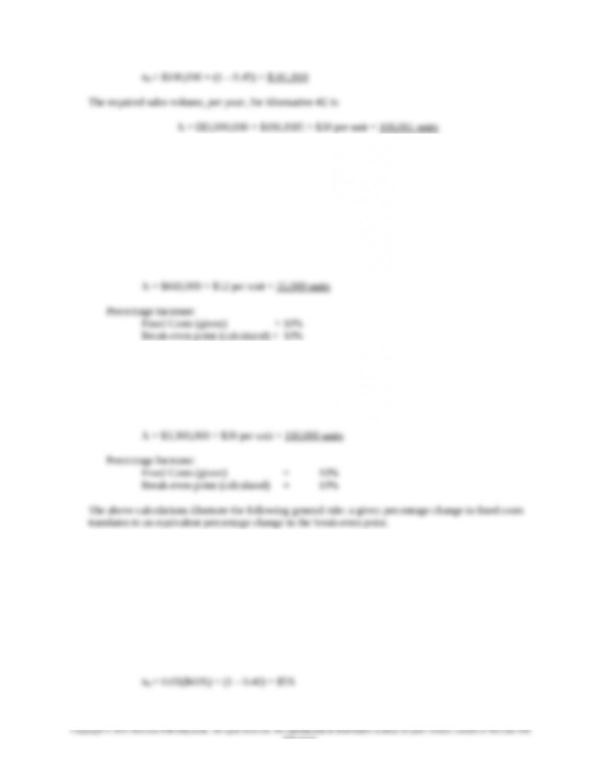
(7) Assume that for the coming year total fixed costs are expected to increase by 10% for each of
the two alternatives. What is the new break-even point, in terms of number of deliveries, for
each decision alternative? By what percentage did the break-even point change for each case?
How do these figures compare to the percentage increase in budgeted fixed costs?
Alternative #1:
New Fixed Costs (per year) = $600,000 × 1.10 = $660,000
New Break-Even Point (in number of deliveries per year):
Alternative #2:
New Fixed Cost (per year) = $3,000,000 × 1.10 = $3,300,000
New Break-Even Point (in number of deliveries per year):
(8) Assume an average income-tax rate of 40%. What volume (number of deliveries) would be
needed to generate an after-tax profit, πA, of 5% of sales for each alternative?
This question is an extension of question 5 (above) to the after-tax case. First, we note (as in 6 above)
that:
πB = πA ÷ (1 – t), where t = effective income-tax rate
For Alternative #1:
9-17
Education.