Unlock document.
This document is partially blurred.
Unlock all pages and 1 million more documents.
Get Access
Chapter 08 - Cost Estimation
An Illustration Cost Estimation: The Use of Regression Analysis in the Gaming Industry
Harrah’s own many large casinos throughout the world, but particular in Las Vegas, where it operates The
Flamingo, Caesars Palace, and Paris Las Vegas. Harrah’s competes in a business that is very focused on
customer satisfaction and customer loyalty. To be more competitive, Harrah’s uses regression analysis
to predict customer satisfaction. The approach is used by many other companies, including UPS and
Google. The five step model below explains how and why Harrah’s uses regression analysis (the story is
described in the book, Super Crunchers, by Ian Ayres, Bantan Books, May, pp 30-32).
The Five Steps of Strategic Decision Making for Harrah’s
1. Determine the Strategic Issues Surrounding the Problem.
Since it operates in a very customer focused business, Harrah’s strategy is to develop and
maintain customer loyalty (a differentiation strategy), and to improve customer profitability.
8-9
Education.

Chapter 08 - Cost Estimation
2. Identify the Alternative Actions:
Harrah’s knows that its customers have a “pain point,” the amount of gaming losses at which the
customer leaves the casino. The casino’s have customer service representatives, called “luck
ambassadors” who are responsible for maintaining customer satisfaction, and in particular, to make sure
the customer does not reach the pain point.
3. Obtain Information and Conduct Analyses of the Alternatives
To obtain information about the pain points of individual customers, Harrah’s began a “Total
Rewards” program that involved a swipeable electronic card that provides certain rewards to customers
but also provides data on the customer’s gaming in the casino. Harrah’s uses this information together
with other information provided by the Rewards customers to develop a regression analysis to predict the
individual customer’s pain point.
4. Based on Strategy and Analysis, Choose and Implement the Desired Alternative
Harrah’s has implemented the regression based system, so that when a given customer is gaming
in the casino (Harrah’s computer system lets it know real-time what the customer is gaming and the gains
or losses for that day) the customer service representatives can be alerted when a given customer is
approaching their predicted pain point, and can be dispatched to urge that customer to take a break, and
perhaps a enjoy free meal at Harrah’s expense.
5. Provide an On-going Evaluation of the Effectiveness of implementation in Step 4.
Harrah’s system requires continuous update for new customers and changes in customer behavior,
so that the regression analyses can be kept current.
8-10
Education.

Chapter 08 - Cost Estimation
Advanced Lecture Notes
There are two advanced lecture notes for Chapter 8. These can be used as handouts or as a basis
for extended coverage of the topics presented in Chapter 8: (1) Time Series Models, and (2) Using the
Beta Distribution in Cost Estimation.
The teaching note on time series models presents an additional method for cost estimation that
can be used when several periods of data are available. Coverage includes an introduction to both simple
trend models and exponential smoothing models. These models present an approach which incorporates
trend (and changes in trend) directly into the estimation model, unlike the high-low method which
presumes a simple linear trend. Simple regression also presumes a simple linear trend, but regression can
be modified using trend variables, dummy variables and other means to adapt to non-linear and changing
trends.
The teaching note on the beta distribution can be used to illustrate how cost estimation models
can be adapted directly for uncertainty in the estimation, much like work measurement and regression are
used to develop statistical measures of the uncertainty in the estimation. This teaching note shows how
the estimation can be developed from probability distributions, using the beta distribution as an example.
The advantage of this approach is the analytical precision of the result, and its usefulness in simulation
studies.
8-11
Education.
Chapter 08 - Cost Estimation
Time-Series Models
An estimation approach which adds further precision to the estimation process is a class of
models called time-series models. Time-series models are prediction models that are developed from
previous observations of the cost to be predicted, without any attempt to examine the relationship of the
cost with any cost driver. Though cost drivers are not considered, time-series models can be very useful
methods for estimating costs, because of their ability to capture non-linear relationships in the data, that
is, seasonality, cyclical movements, and different types of trends. There are a number of time-series
models; the two types of models we will consider are among the most commonly employed:
a) Simple trend models
b) Exponential smoothing models
Simple trend models are based only on recent periods' data, and there is no statistical or explicit
decomposition into seasonality, cycles or trends. The advantage of the methods is they are easy to
calculate. The simplest of these is the model which says that the next period will be the same as the prior
period. A more common and more useful variation is called the period-to-period-change (PTP) model.
The period-to-period-change model is based upon the average change in the cost over two or more prior
periods. To explain this model we will need to adapt our notation for the predicted value, so that
represents the predicted value for period T. The PTP model in its simplest form is calculated as follows:
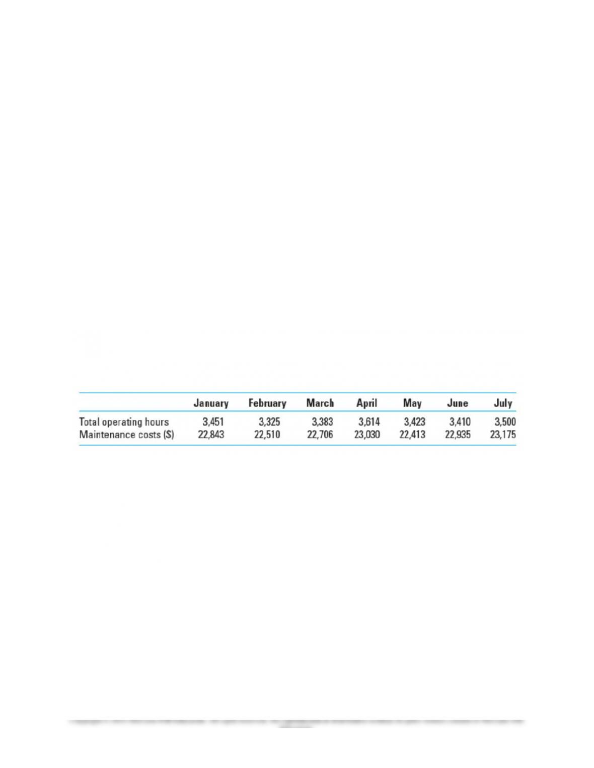
Using this approach we can estimate August maintenance cost for Ben Garcia (data in Exhibit 8-1):
$23,175 + ($23,175 - $22,935) = $ 23,415
Since this method incorporates only the two most recent years, the estimation reflects the upward
trend for these two years. It is also possible to use all prior years' data available, and then the equation
would look like this (where n is the number of periods of data):
8-12
Education.

Chapter 08 - Cost Estimation
The above approach weights each prior period equally in the estimation. Management
accountants can weight the more recent periods more heavily, if desired, by multiplying each term in the
numerator by a weighting constant (often chosen to be simply 1,2,3..., from least to most recent period)
and adjusting the denominator accordingly (the denominator is now the sum of the weights). However, if
management accountants choose an unweighted model, as above, then the calculations can be simplified
as follows:
The estimated amount of maintenance cost for August using the unweighted model in the above
equation would be:
$23,175,000 + ($23,175 - $22,843)/6 = $23,230.
Exponential smoothing. While the PTP model can be adapted for weighting the most recent
years' data, the exponential smoothing approach integrates both weighting and an iterative calculation to
"smooth" the data. Exponential smoothing, sometimes referred to as "adaptive forecasting,” is based upon
a weighted moving average of past data. Because the calculations can be tedious, this approach is
typically implemented in either spreadsheets or specialized software.
Though exponential smoothing can be implemented in a variety of ways, a common approach is
to separate two of the components of the time-series modelthe trend to the data and the fluctuations
about the trend. A smoothed value is computed for each component and the product is the estimated
value:
Estimated Cost (August) = Smoothed Cost Trend (July) x Smoothed Cost (July)
The term "smoothing" describes this method's use of a weighting constant, a, together with a
smoothing function, S(Y), to develop the smoothed estimation. The weighting constant (a) is a number
between zero and one, such that the closer a is to one, the more weight is given to recent periods in the
data, and vice versa. The smoothing function is employed such that the smoothed value at the time T is a
linear combination of the actual value at time T and the smoothed value of the previous period:
Beginning with period one, the smoothing function is calculated for each period, and iteratively,
the final estimation for the desired future period is derived. Exponential smoothing is a widely used
technique that, with a studious choice of the weighting function, can provide management accountants
with accurate estimates.
The calculations for the maintenance cost data are as follows, beginning with February since a
smoothed value cannot be obtained for the period year in the series:
Smoothed (February) = ½ actual cost (February) + ½ actual cost (January)
= ½ x $22,843 + ½ x $22,510 = $22,676.5
Smoothed (March) = ½ actual cost (March) + ½ smoothed (February)
= ½ x $22,706 + ½ x $22,676.5
8-13

Chapter 08 - Cost Estimation
The remaining smoothed values for the annual costs are shown in Exhibit 1.
The smoothed values for the trend of the series are obtained as follows, beginning with March,
since the smoothed trend cannot be obtained for the first two years in the series:
Smoothed Trend (March) = ½ {actual(February)/actual(January)} +
½ {actual(March)/actual(February)}
The smoothed values for the trend of the costs are shown in Exhibit 1. The Smoothed prediction
for August is thus:
Estimated Cost (August) = Smoothed Cost Trend (July) x Smoothed Cost (July)
= 1.008 x $22,980.45 = $23,164.29
Exhibit 1: Calculation of Smoothing Function for Maintenance Cost Data
Month SMOOTHED TREND SMOOTHED COST
Jan. --- ---
Feb. --- ½(22,510) + ½ (22,843) = $2,676.5
March ½(22,706/22,510) +1/2(22,510/22,843)
= .997
½(22,706) + ½(22,767.5) = $22,691.25
April ½(23,030/22,706) + ½(.997)
= 1.006
½(23,030) + ½(22,2691.25) = $22,860.63
May ½(22,413/23,030) + ½(1.006)
= .989
½(22,413) + ½(22,860.63) = $22,636.82
June ½(22,935/22,413) + ½(.989)
= 1.006
½(22,935) + ½(22,636.82) = $22,785.91
July ½(23,175/22,935) + ½(1.006)
= 1.008
½(23,175) + ½(22,785.91) = $22,980.45
8-14
Education.

Chapter 08 - Cost Estimation
Using The Beta Distribution In Cost Estimation
Another approach for assessing uncertainty in a cost estimate, the probabilistic approach, is
similar to the statistical methods of work measurement and regression described in the chapter. The
difference is that the estimates are obtained from expert judgements rather than from observations of the
activity.1 A common way to employ the method is to use the beta distribution. In this technique, the
expert is asked to give three time estimates for the activity in questionthe lowest, the most likely, and
the highest cost estimate. For example, if we were estimating the labor time in a manufacturing activity,
we might estimate the times as follows:
Shortest time (S): 3 minutes
Most likely time (M): 4 minutes
Longest time (L): 6.5 minutes
Using the beta distribution approach, it is possible to obtain the mean and variance of the
distribution directly from these estimates, as follows:
Mean time: (S + 4xM + L)/6 = (3 + 4x4 + 6.5)/6 = 4.25 minutes
Variance:
The mean and variance are interpreted here in the same manner as in the standard error in
regression - the mean of 4.25 minutes is the single best prediction of the average time over repeated
observations (in contrast, the "most likely time" of any single observation is 4 minutes), and the variance
of .583 minutes is a measure of the uncertainty in the prediction.
A limitation of the probabilistic approach using the beta distribution is that the beta distribution
does not have a well-known form (normal, binomial, etc), so we cannot go to a table and find the bounds
of the confidence interval, as in work measurement. However, as is often the case, if we are interested in
the sum of estimates of the time for a number of activities, then the central limit theorem can apply, and in
this case, the mean for the sum of the activities is the sum of the individual means as computed above,
and the variance of the sum is also the sum of the individual variances as computed above. Moreover, the
mean and variance of the sums obtained in this manner will follow the properties of the normal
distribution, so that we can use the tables for the normal probability function and identify confidence
intervals as in work measurement above. In summary, the probabilistic approach allows us to develop
confidence intervals on prediction accuracy based upon experts' judgments about the likely times or
inputs to an activity.
1 1 This method is explained in an article by Edwin A. Wood and Robert G. Murdick, "A Practical Solution to


