Chapter 04 – Job Costing
4-46 (Continued -1)
h. Selling& Administrative Expense 2,400
Accumulated Depreciation 2,400
i. Advertising Expense 5,500
Cash 5,500
j. Factory Overhead 13,500
Cash 13,500
k. Selling & Administrative Expense 13,250
Cash 13,250
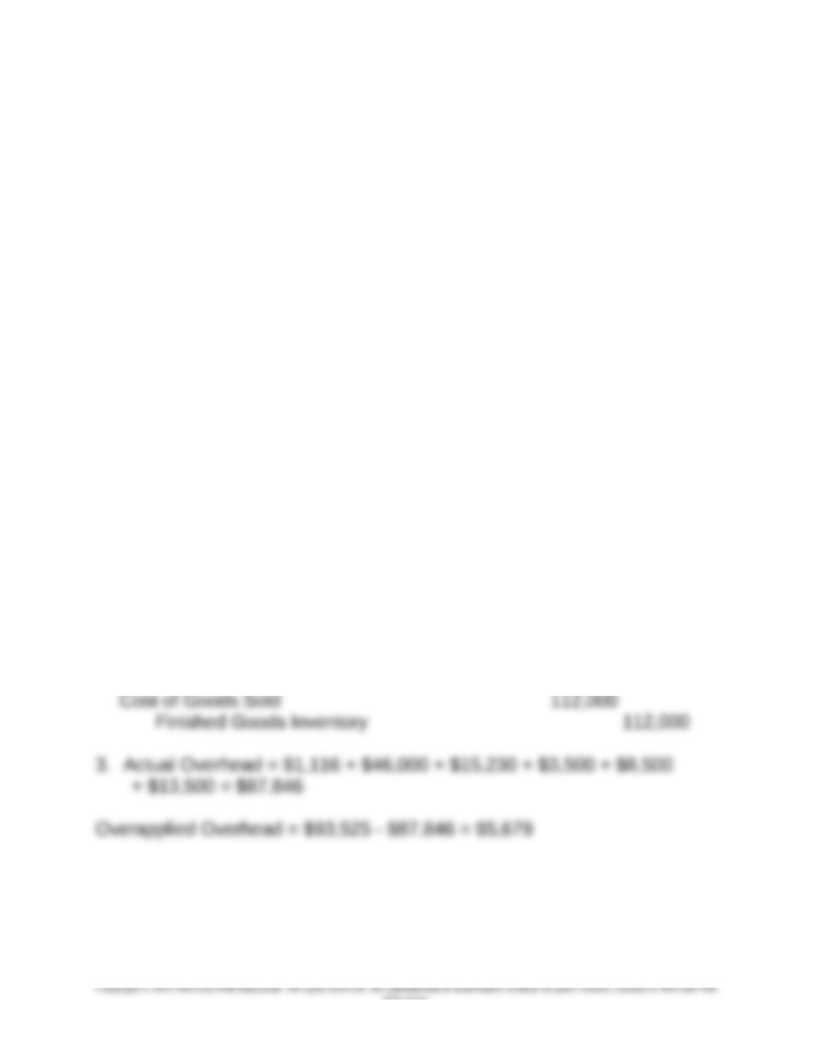
l. Applied Overhead = $14.50 x 6,450 DL hour = $93,525
Work-in-Process Inventory 93,525
Factory overhead 93,525
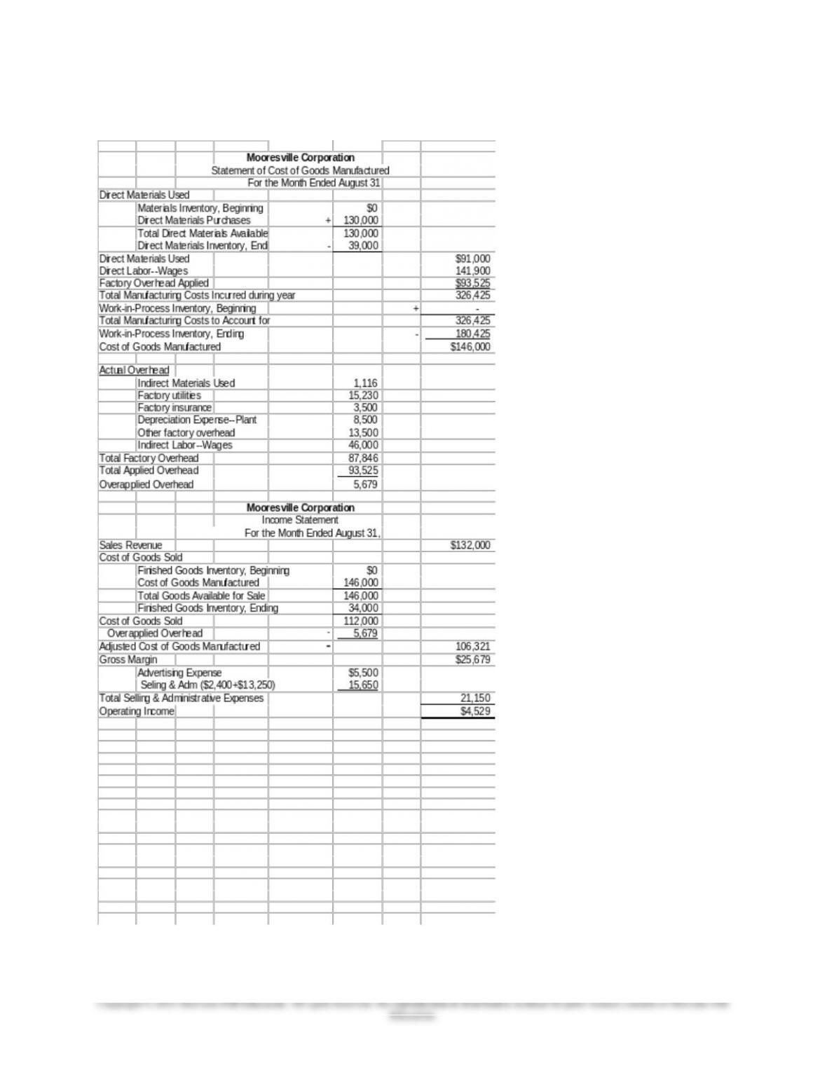
m. Finished Goods Inventory 146,000
Work-in-Process Inventory 146,000
n. Accounts Receivable 132,000
Sales Revenue 132,000
4-31
Education.
Chapter 04 – Job Costing
4-46(Continued -2)
4.,5.
4-32
Chapter 04 – Job Costing
4-47 Application of Overhead (15 min)
1. $2,720,000 ÷ 1,700,000 = 160% of professional labor cost
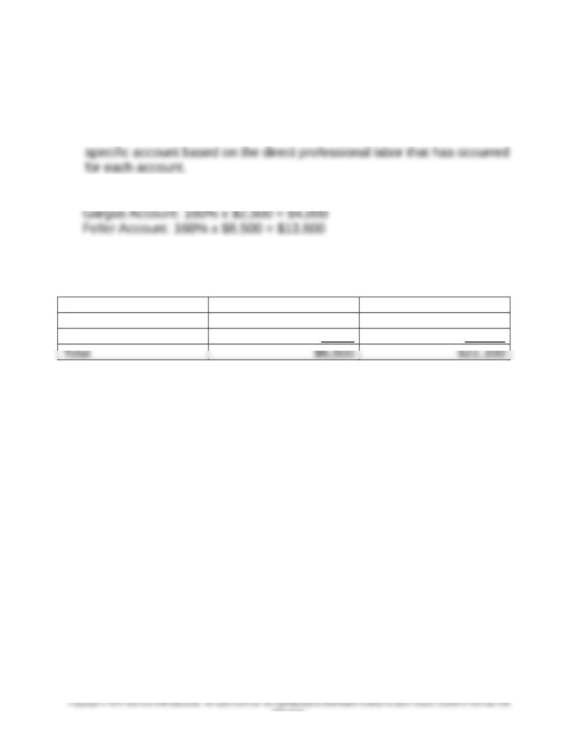
This is used to allocate the budgeted overhead for the period to each
2. Amount of overhead charged to:
3. Computation of the total contract cost:
Cost Gargus Account Feller Account
Direct Labor $2,500 $8,500
Overhead 4,000 13,600
Total $6,500 $22,100
4-33
Education.
Chapter 04 – Job Costing
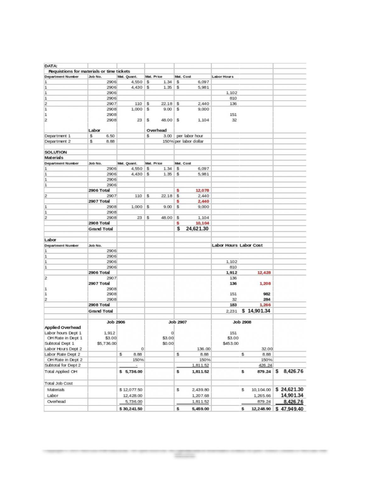
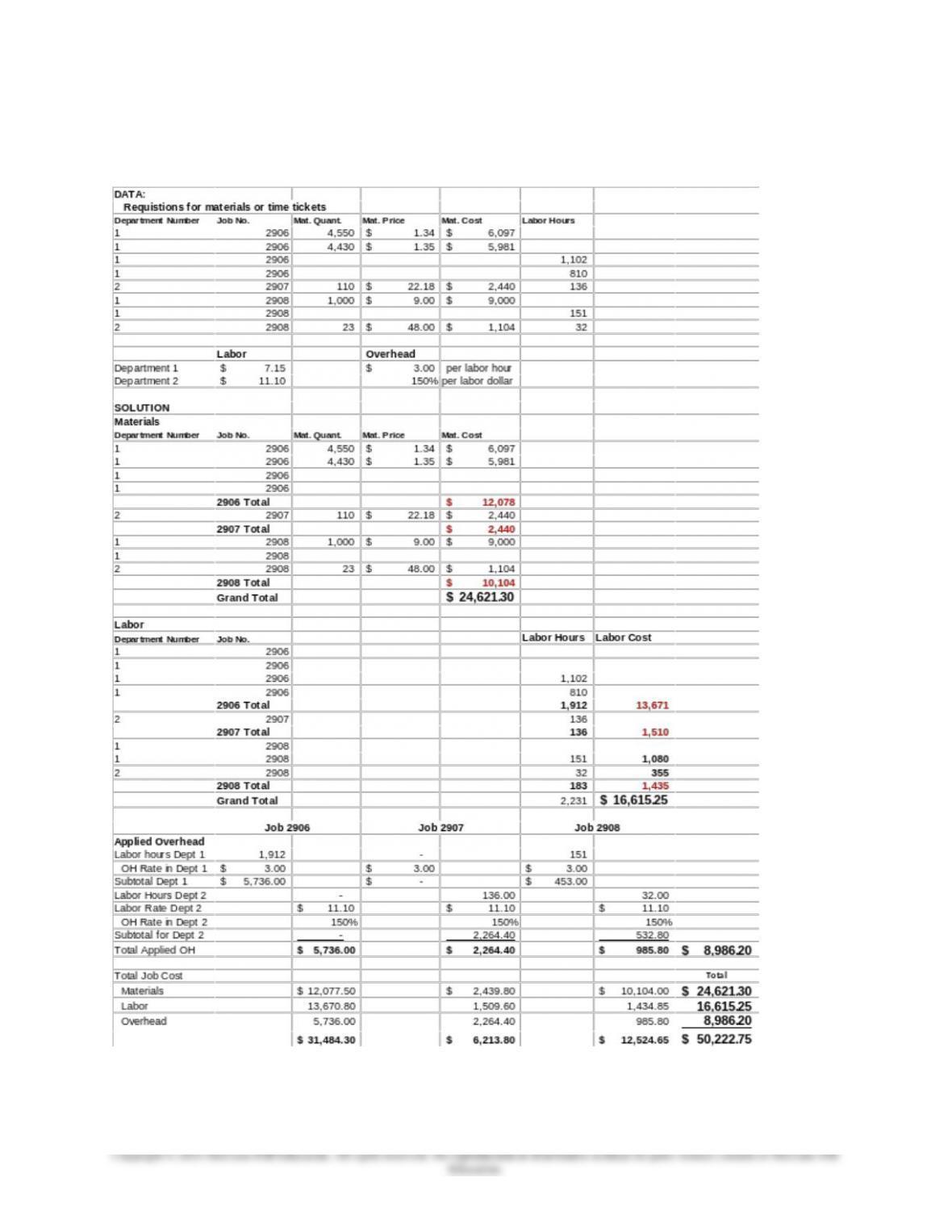
4-48 Job Cost; Spreadsheet Application; Pivot Tables (50 min)
1.
4-34
Chapter 04 – Job Costing
4-48 (Continued -1)
2. The solution for requirement two is shown below
4-35

4.48 (continued -2)
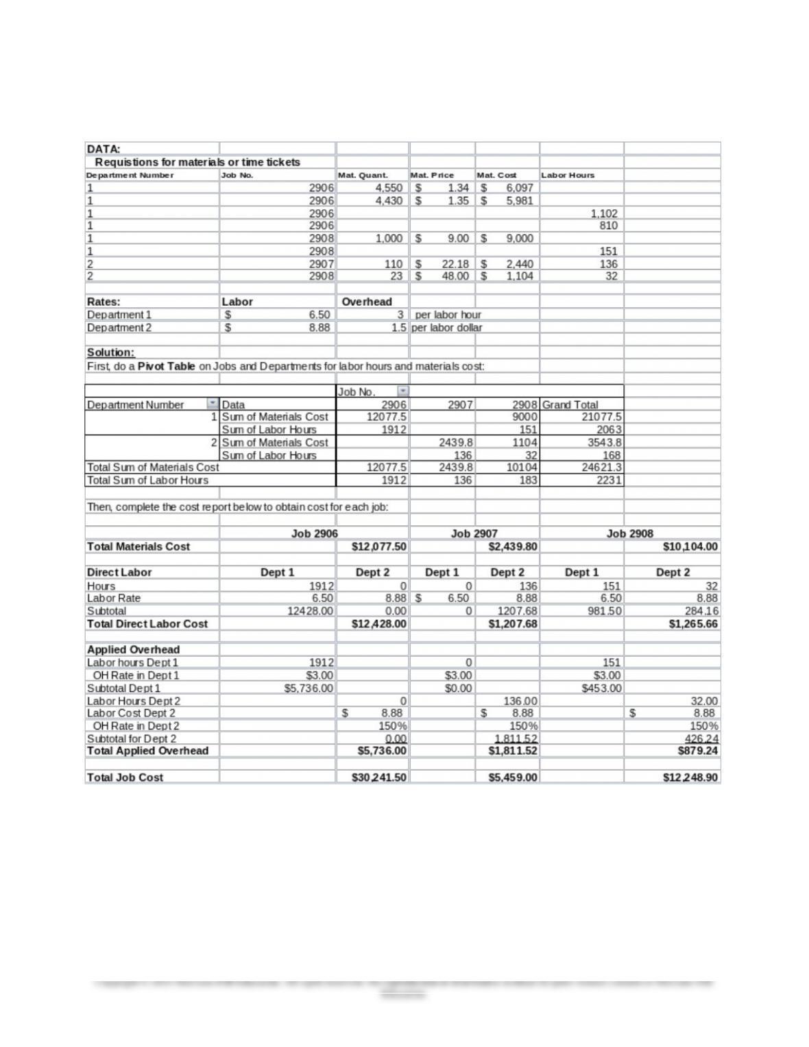
3. Using Pivot Tables in Excel provides the flexibility to easily manipulate
the data to find summary information from the data. The solution for Part
3, identical to that in Part 1, but using Pivot Tables (see tutorial for Pivot
Tables at the end of the solution for 4-49 and in the Excel Tutorials on
the text Web site):
4-36
Education.
Chapter 04 – Job Costing
4-48 (continued -3)
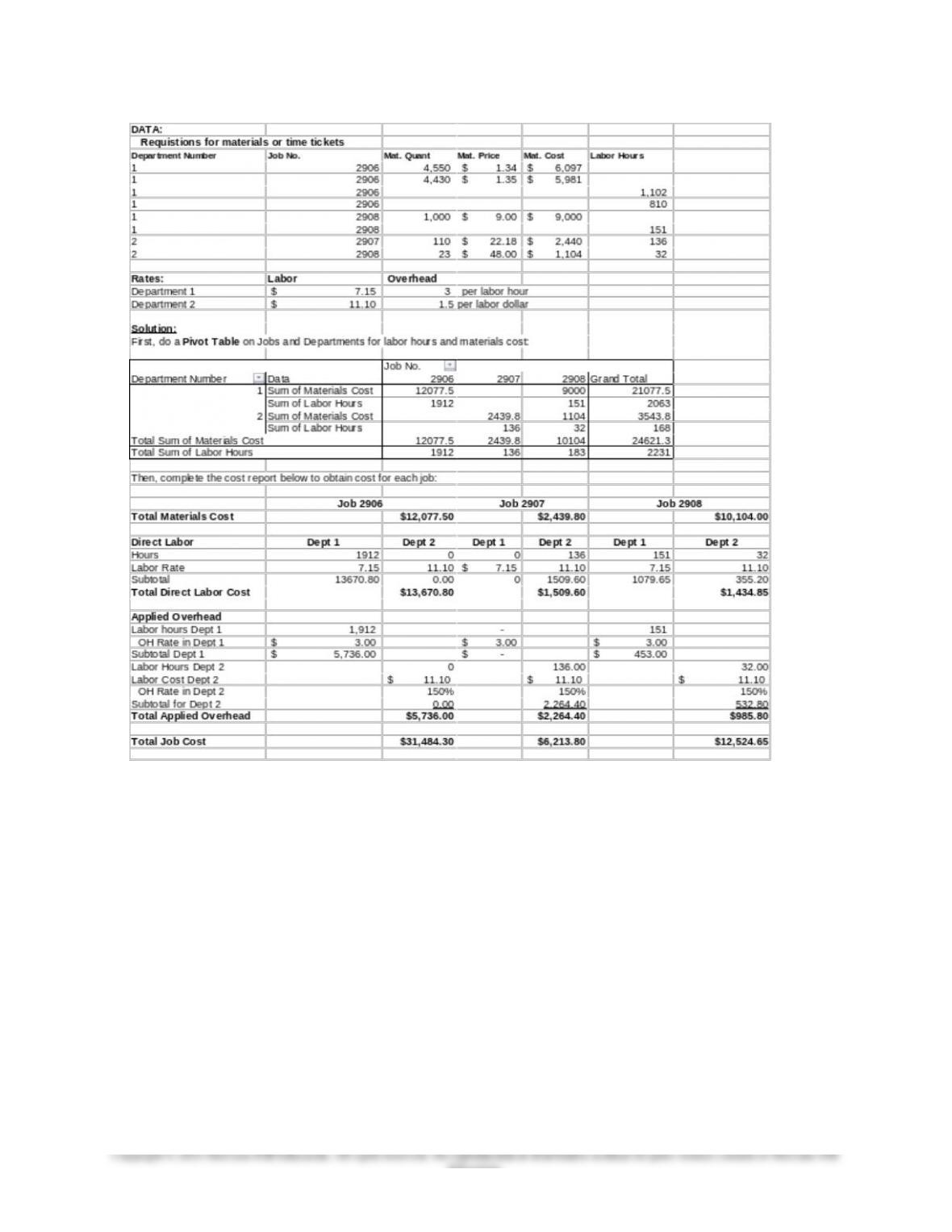
4. Using Pivot Tables in Excel provides the flexibility to easily manipulate
the data to find summary information from the data. The solution for Part
4, identical to that in Part 2, but using Pivot Tables:
4-37
Chapter 04 – Job Costing
4-38
Education.
Chapter 04 – Job Costing
4-48 (continued -4)
Tutorial and Illustration:
Creating and Using Pivot Tables—the following steps can be used to
create a pivot table that in turn, can be used to evaluate various data sets
with ease. By exploring the pivot tables within Excel you can use this
feature to perform many different summations and calculations. This
tutorial will only show you a simple version of a pivot table. The data for
the tutorial is taken from the self-study problem at the end of the chapter,
the Watkins Machinery Company broken down into further information for
hypothetical separate dates and amounts.
1. Enter the data for the problem into a spreadsheet, as follows (the
first two columns are the same, the reason for which will be clear
in the solution to follow):
Purchased Product Purchased
Product
Date Amount Applied to:
Indirect Materials Indirect Materials 02/26/16 $ 3,000 Indirect
Indirect Materials Indirect Materials 03/01/16 1,250 Indirect
Material Y Material Y 03/03/16 800 Job 101
Material Y Material Y 03/04/16 1,600 Job 102
Material X Material X 03/06/16 1,200 Job 101
Material X Material X 03/08/16 1,600 Job 102
Indirect Materials Indirect Materials 03/10/16 1,250 Indirect
Material X Material X 03/11/16 800 Job 101
Material X Material X 03/11/16 2,000 Job 101
Material X Material X 03/12/16 1,000 Unapplied
Material X Material X 03/20/16 1,000 Job 101
Material Y Material Y 03/20/16 2,000 Unapplied
Material Y Material Y 03/24/16 900 Job 102
Material X Material X 03/24/16 1,400 Job 102
Material Y Material Y 03/25/16 200 Job 101
Material Y Material Y 03/26/16 1,000 Unapplied
Indirect Materials Indirect Materials 03/26/16 1,250 Indirect
4-39
Education.
4-48 (continued -5)
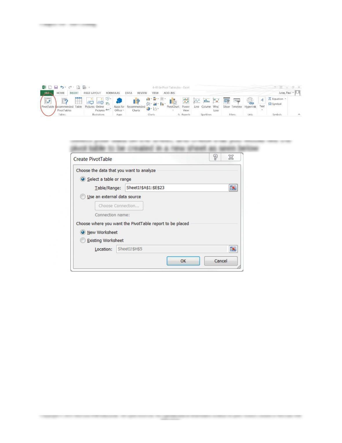
2. Go to the Insert tab on the ribbon, and select the PivotTable
button. You can choose Pivot Table or Pivot Chart; choose Pivot
Table.
3. Once you have selected PivotTable a new screen will pop-up.
4. Now you can click OK.
5. As you can see, your pivot table is shown within a new sheet, and
now a new box has opened on the right side of your screen. This
box allows you to modify the data within Excel. The lists shown in
the Fields box are the headers of your data columns in the “Data”
sheet. You should now select the field names, and drag them into
the boxes below. For a detailed example see the screen capture
on the following page:
4-40
Education.