Chapter 18 – Strategic Performance Measurement: Cost Centers, Profit Centers, and the Balanced Scorecard
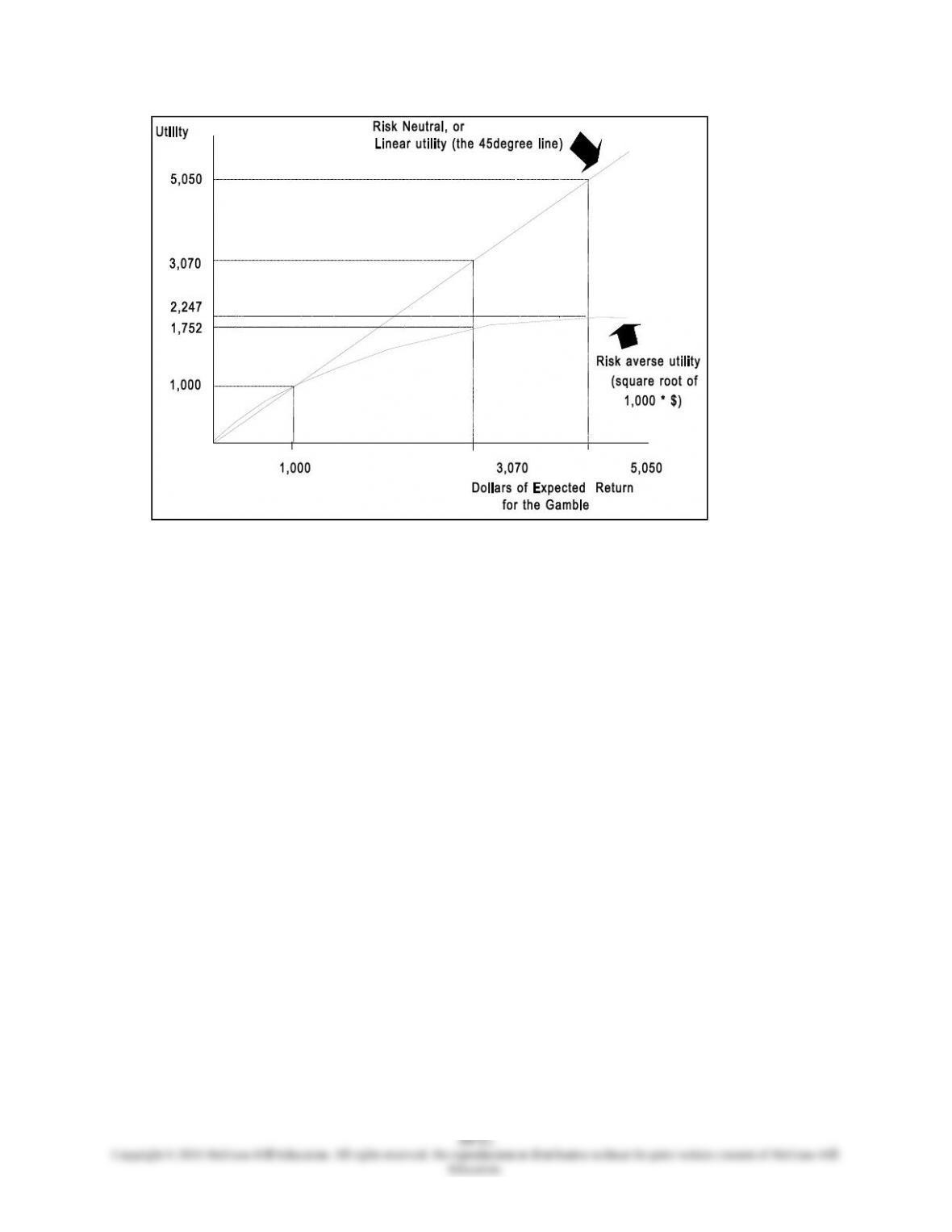
Exhibit 2: Risk Neutral and Risk Averse Utility Functions
Using mathematical transforms such as the square root or the logarithm of the dollars of expected
return provides a practical approach for representing risk-averse utility curves. When developing
incentive plans, the management accountant will consider tools such as this to provide the proper
motivation for the manager. The motivation is important to provide the incentive for both (a) a high level
of effort by the manager and (b) to provide a reward scheme which will cause the manager’s decisions to
be congruent with those of the relatively less risk-averse top management.
The Role of Information and Risk Preferences in Decision Making
The note explains the role of information and risk preferences in decision making. The first step is to
understand how the value of information is determined. To do this, we adopt the widely used decision
model based upon expected valuesdecision analysis. Decision analysis provides a systematic approach
for a decision maker to determine the best of a set of choices, when the outcome of the choices is
uncertain. The criterion for choice is maximum expected utility, where utility is typically measured in
dollars. For simplicity, we will hereafter (except where otherwise noted) refer to utility in terms of dollars,
and use the criterion, “expected value.” For example, if for a given choice the decision maker faced two
outcomes, one with a value of $10 and the other with a value of $50, and the outcomes were equally
likely, then the expected value of the choice would be:
Expected Value = .5 x $10 + .5 x $50 = $30
Using this expected value measure, the decision maker would rank order the choices available and
choose the option with the greatest expected value. The role of information in this context is to improve
the expected values available to the decision maker by updating the odds, that is, updating the
probabilities for the different outcomes.
To illustrate, we develop the decision analysis for a manager who oversees the subcontractors who
provide services to a large construction company. The subcontractors perform certain services and then

Chapter 18 – Strategic Performance Measurement: Cost Centers, Profit Centers, and the Balanced Scorecard
bill the construction company. The manager must decide which, if any, of the bills submitted for payment
to the company are in error (usually including over-charges), and should be corrected. The uncertainty lies
in the fact that the manager does not know, prior to an extensive investigation of each bill, whether it is in
error or not. The manager can perform an investigation of the bill, which the manager estimates on the
average would cost $100, and when needed, a correction of the bill, which on the average would cost an
additional $100. Alternatively, the manager could let the bill pass and hope for the best. If the bill is in
error, the company will (unknowingly) pay for the overcharges, which will on the average be about
$1,000 per bill. We will call this the “cost of incorrect acceptance.” From experience, the manager knows
that the odds of an incorrect bill are about one in ten. However, without conducting an investigation, the
manager has no way of knowing which bill is in error, so that the best strategy for investigation will either
be to investigate all the bills, none of the bills, or perhaps some randomly selected sample. This decision
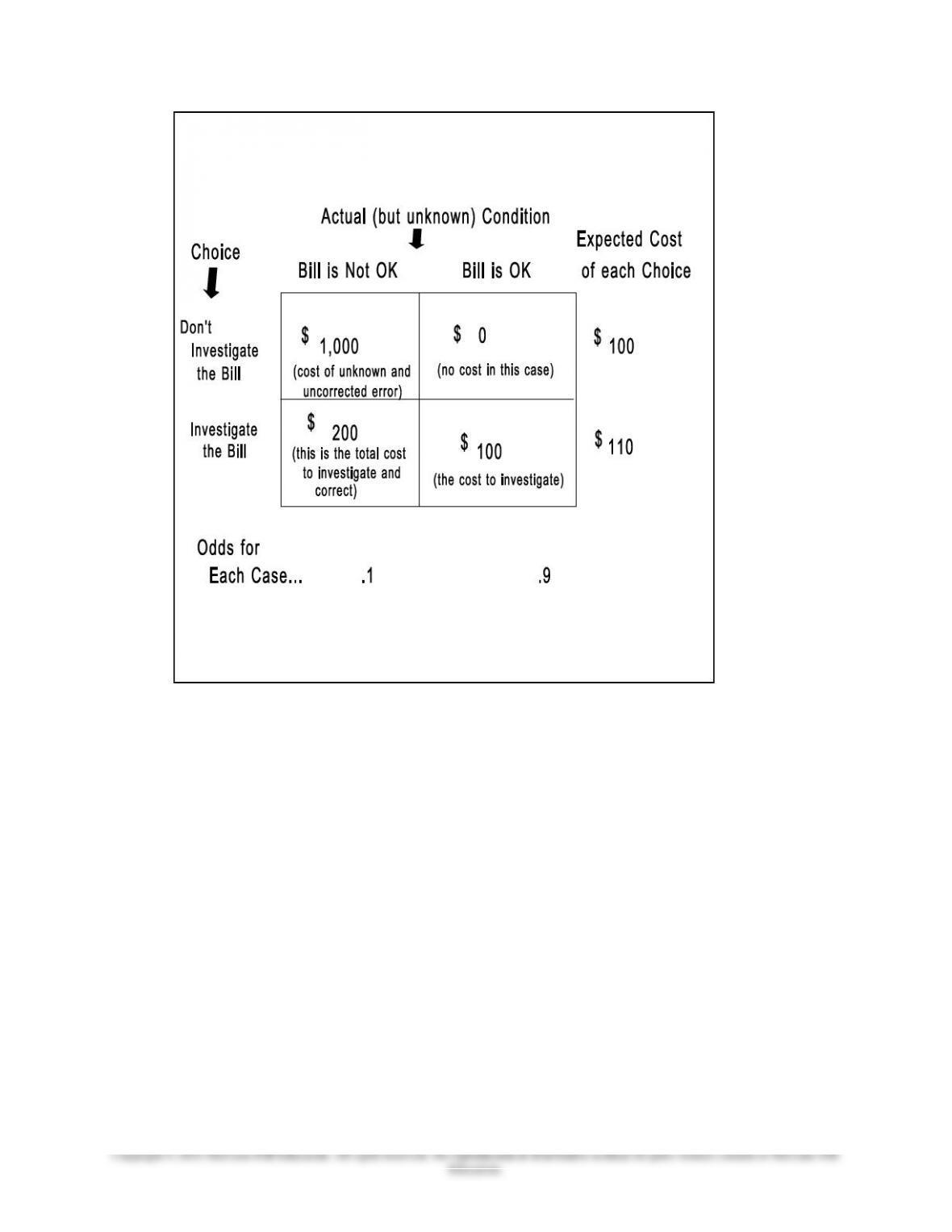
problem can be formalized, as is illustrated in Exhibit 1.
The manager wants to choose the option that will be least costly to the firm, and in this case, the
lowest expected cost is to accept each bill without investigation. This would produce an average cost of
$100 (one-tenth of the bills are in error by $1,000). The alternative “investigate and correct” strategy
would be more costly on the average, or $110 per bill (a total investigate and correct cost of $100 + $100
= $200 which is incurred one-tenth of the time, and the cost to investigate only, $100, the rest of the time;
for a total expected cost of .1 x $200 + .9 x $100 = $110).
After some experience with this decision setting, the manager can develop a simplified decision rule,
the “threshold ratio,” which is calculated as follows.1 The decision rule is to investigate a bill when the
odds that it is not-OK is greater than the threshold ratio. For this data, the threshold ratio is one-ninth,
which is determined from the ratio of the three different costs as follows:
Cost of Investigation
Threshold Ratio =
Cost of Incorrect Acceptance, less Cost of Correction
= $100/ ($1,000 – $100)
= 1/9
1 The decision rule is developed as follows. Let P = the probability of the not-OK condition, a = cost of
investigation, b = cost of correction, and c = cost of incorrect acceptance. Then, the manager will choose to
investigate if the expected cost of investigating is less than the expected cost of not investigating:
(a + b) x P + b x (1 – P) < c x P
or: p > b/(c – a)
18-12
Education.
Chapter 18 – Strategic Performance Measurement: Cost Centers, Profit Centers, and the Balanced Scorecard
Exhibit 1: The Value of Information in a Simple Decision Problem
The manager compares the threshold ratio to the odds for an incorrect bill to determine whether to
begin an investigation. Since the threshold ratio is less than the odds of the not-OK bill (1/10 is less than
1/9), the best decision is not to investigate.
The Role Of Information
Up to this point we have assumed that the manager knows only the proportion of bills in error, but
does not have information to identify those specific bills that are in error. This information would be
useful to the manager, as a means to reduce overall investigation, correction, and incorrect acceptance
costs.
Suppose the manager has access to a report in which accounting information is used to prepare a
“risk score,” which would perfectly identify the bills that are in error, so that the manager could avoid the
mistakes of incorrect acceptance and incorrect rejection for any given invoice. The risk score could be
developed from information about the biller’s accounting system (cash or accrual-based, the quality of the
internal accounting control system, whether or not there is an internal audit function, how product costs
are calculated, etc.). For example, the risk score might be the sum of the relevant risk factors noted for the
invoice, where the number of possible risk factors is 35, and the average number of risk factors noted for
the typical invoice is usually between 12 and 24. While it is unlikely such a score would perfectly signal
the true error condition, as we assume here, the assumption is useful for this simplified illustration.
18-13

Chapter 18 – Strategic Performance Measurement: Cost Centers, Profit Centers, and the Balanced Scorecard
With perfect information, the manager would be able to always choose the lowest cost outcome
(when there is an error, investigate and correct the bill; when no error, accept the bill). With perfect
information, the manager’s expected cost is simply the sum of the expected costs for each possible
outcome, given the best choice for each error condition: .1 x $200 +.9 x $0 = $20. With perfect
information, the manager will not conduct an investigation if the information reports there is no error in
the bill, and similarly, there is no possibility the manager will incorrectly accept a bill that is in error.
The value of the information, then, is the differential, $100-20 = $80, the difference between the expected
cost to the manager with and without the perfect information. This is called the expected value of perfect
information. It is called the expected value of perfect information because, while the manager can prevent
mistakes in identifying which bills have errors, the manager cannot prevent the occurrence of errors,
which has a probability of 10% for each invoice.
The expected value of perfect information is a useful concept for measuring the value of information.
It is particularly appealing in accounting, because it shows directly the maximum potential benefit to a
decision maker from receiving information that will reduce some of the uncertainty in the decision
setting.
Obtaining Probabilities from the Normal Probability Curve
Implementing the above decision rule will require the manager to estimate the costs of investigation,
correction, and incorrect acceptance, and to estimate the probabilities that a given invoice will be in one
of the two conditionsOK or not-OK. This section explains how the normal probability curve can be
used to facilitate development of the probability estimates.
The first step in using the normal curve would be for the manager to maintain a “history” of the risk
scores of selected invoices for a given period, together with the outcome of whether the invoice was in
error or not. In this way the manager develops two frequency distributions, one for each error condition
that shows the frequency of all the different possible risk scores that are observed under that error
condition. Assuming that the method of calculating the risk score is useful and effective, invoices with
higher risk scores will more likely be in error than other invoices, and given a sufficiently large number of
invoices, the pattern will likely follow that of the normal curve for each error condition, as illustrated in
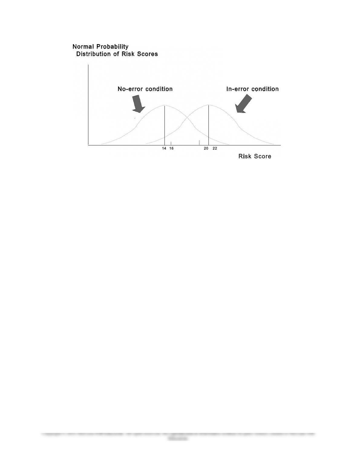
Exhibit 2.
Now, given the historical data in these two frequency distributions, it is possible for the manager to
develop a revised, more accurate probability estimate based upon the risk score of each invoice. To
illustrate, consider Exhibit 2, wherein the no-error distribution is assumed to be approximately normally
distributed with a mean risk score of 14 and a standard deviation of 4; similarly, the in-error distribution
has a mean of 22 and a standard deviation also of 4. Suppose that the manager observes that a given
invoice has a risk score of 16. Because the risk score is relatively low, the probability estimate that the
invoice is in error also should be low. Rather than to determine this estimate judgmentally, the manager
can use the information in the two historical distributions to obtain a quantitative estimate.
18-14
Chapter 18 – Strategic Performance Measurement: Cost Centers, Profit Centers, and the Balanced Scorecard
Exhibit 2: Normal probability distribution of Risk Scores
The first step is to obtain the probability for the point 16, by converting the value for 16 to a
standard normal value, which can then be found in tables for the standard normal curve. The conversion
of any point to a standard normal value is done by subtracting the mean of the normal distribution from
the value of the point, and then dividing by the standard deviation of the curve, as follows:
Standard normal equivalent for point 16 = (mean-16)/Standard deviation
To illustrate, since the mean of the in-error distribution of risk scores is 22, and the standard
deviation is 4, the standard normal equivalent for the point 16 would be, from the above formula:
(16-22)/4 = -1.5
Since the normal curve is symmetric, we can ignore the negative sign and go directly to a table of
normal probabilities, Exhibit 3, to find that the probability for the in-error condition at the point 16 is .
1295.
Similarly, the probability of the point 16 for the distribution of no-error risk scores can be found
from the mean (14) and standard deviation (2) of the no-error distribution, where the standard normal
value is (16-14)/4 = .5 and, from Exhibit 3, the probability for the no-error distribution at the point 16 is .
3521.
18-15

Chapter 18 – Strategic Performance Measurement: Cost Centers, Profit Centers, and the Balanced Scorecard
Risk Score Standard Normal Probability
.5 .3521
1.0 .2420
1.5 .1295
2.0 .0539
2.5 .0175
3.0 .0044
Exhibit 3: Values of the Standard Normal Probability Function
Now, the manager’s best estimate that the invoice with the 16 risk score is in error is given by the
ratio of the in-error to total probabilities, as follows:
.1295/(.1295 + .3521) = .2688
and the probability that the invoice is not in error is
1.0 – .2688 = .7312
Thus, the manager knows that based upon the favorable risk score, this invoice has a relatively
small chance of being in error. Without the risk score information, the manager’s best guess would be that
this invoice would have the same probability of being in error as for any other invoice, or 10%, since one
in ten invoices historically turn out to be in error. The risk score, and the use of the normal probability
curves, can significantly improve the manager’s estimate of the probabilities. For practice now, determine
the in-error probability for an invoice with a risk score of 20.2.2
In summary, what the manager has accomplished is to use the historical frequency data for risk
scores under each error condition to form a normal probability curve for each error condition, which then
can be used to better estimate the specific probability that a given invoice will be of either condition,
based upon the invoice’s risk score.3
The normal curve can be used in a variety of contexts such as this, where there is prior data or
experience available to develop a probability distribution from which the probability of any specific value
can be determined, as in the above illustration.
The Effect Of Risk Preferences On Decision-Making
The manager’s decision rule as presented above is a useful model for illustrating the role of risk
preferences in decision-making.
22 The standard normal value for the in-error condition is (20-22)/4 = .5, with a related probability of .3521. The
standard normal value for the no-error condition is (20-14)/4 = 1.5, with a related probability of .1295. The
probability of the invoice being in error is thus .3521/(.3521 +.1295) = .7312.
33 It is also possible for the manager to incorporate prior probability beliefs in this analysis, and to perform a
Bayesian analysis in a similar fashion. The Bayesian approach for this particular context is best illustrated by
Thomas R. Dyckman, “The Investigation of Cost Variances,” Journal of Accounting Research, Fall 1969, pp 215-
244.
18-16
Education.

Chapter 18 – Strategic Performance Measurement: Cost Centers, Profit Centers, and the Balanced Scorecard
The following illustration shows how risk preferences can produce an undesirable decision.4
Suppose the manager has the option to invest $25,000 in either a new manufacturing technology which
could improve the efficiency of the plant considerably, or alternatively, to spend the $25,000 in the
redesign of one of the product lines. The difference is that there is a substantial risk that the new
technology will not work, and relatively little risk that the product re-design will produce modest returns.
Suppose there is a 30% chance that the new manufacturing technology will produce a $100,000 savings in
plant costs, and a 70% chance of only a $20,000 savings. Also, the product re-design will produce with
fifty-fifty odds either a savings of $50,000 or a savings of $30,000. The manager will earn 15% of the net
savings generated from either investment, since managers’ compensation is based in part on a bonus of
15% applied to earnings before tax.
Suppose that top management of the entity has a risk-neutral approach to the decision problem
(i.e, linear expected utility in dollars), then top management would prefer the new manufacturing
technology over the product re-design, because of the higher expected value ($19,000 and $15,000
respectively). This is illustrated as follows:
Top Management’s Decision Analysis:
Expected Value of Investing in New Manufacturing Technology
(.3 x $100,000 + .7 x $20,000 = $44,000) – $25,000 = $19,000
Expected Value of Investing in Product Re-design
(.5 x $50,000 + .5 x $30,000 = $40,000) – $25,000 = $15,000
While the choice is clear to top management, the manager who is risk-averse has a different view.
First, we must describe the manager’s utility function. One way to describe a risk-averse utility function is
to use the square-root transform.5 Then, suppose the manager’s utility function can be described by the
square root of the amount, “dollars received times 100″ (the multiplication times 100 is a simple scale
factor to produce meaningful amounts). Then, the manager’s decision analysis can be illustrated as
follows:
The Manager’s Decision Analysis
Expected Utility of Investing in New Manufacturing Technology
Expected Utility of Investing in Product Re-design
It is clear that the manager has higher utility for the product re-design. The square root utility
function deflates the potentially high return of the new manufacturing technology investment, and the re-
44 This example is found in the article by Chee W. Chow and William S. Waller, “Management Accounting and
Organizational Control,” Management Accounting (April 1982), pp36-41.
55 The square root function reduces the outcome in dollars by an increasing proportion of the size of the amount,
and thus is a good proxy for risk aversion. That is, under uncertainty, the decision maker places a lower value on the
larger amounts in preference for smaller, more certain amounts.
18-17
Education.

Chapter 18 – Strategic Performance Measurement: Cost Centers, Profit Centers, and the Balanced Scorecard
design project has higher expected utility, if not higher expected monetary value. From top
management’s perspective, the 15% bonus incentive has dysfunctional consequences. Management should
therefore consider amending the pay plan to reduce the effect of the bonus scheme on managers’ decision-
making.
Assignments For Supplementary Material
Question 1: Decision Making (CMA adapted)
Video Recreation Inc. (VRI) is a supplier of video games and video equipment such as large-
screen televisions and video cassette recorders. The company has recently concluded a major contract
with Sunview Hotels to supply games for the hotel video lounges. Under this contract, a total of 4,000
games will be delivered to Sunview Hotels throughout the western United States, and all of the games
will have a warranty period of one year for both parts and labor. The number of service calls required to
repair these games during the first year after installation is estimated as follows.
Number of
Service Calls Probability
400 .1
700 .3
900 .4
1,200 .2
VRI’s Customer Service Department has developed three alternatives for providing the warranty
service to Sunview; these three plans are presented below and in the next column.
Plan 1
VRI would contract with local firms to perform the repair services. It is estimated that six such
vendors would be needed to cover the appropriate areas and that each of these vendors would charge an
annual fee of $15,000 to have personnel available and to stock the appropriate parts. In additional to the
annual fee, VRI would be billed $250 for each service call and would be billed for parts used at cost plus
a 10 percent surcharge.
Plan 2
VRI wold allow the management of each hotel to arrange for repair service when needed and then
would reimburse the hotel for the expenses incurred. It is estimated that 60 percent of the service calls
would be for hotels located in urban areas where the charge for a service call would average $450. At the
remaining hotels, the charge would be $350. In addition to these service charges, parts would be billed at
cost.
Plan 3
VRI would hire its own personnel to perform repair services and to do preventive maintenance.
Nine employees, located in the appropriate geographical areas, would be required to fulfill these
responsibilities, and their average salary would be $24,000 annually. The fringe benefit expense for these
employees would amount to 35 percent of their wages. Each employee would be scheduled to make an
average of 200 preventive maintenance calls during the year; each of these calls would require $15 worth
of parts. Because of this preventive maintenance, it is estimated that the expected number of hotel calls
for repair service would decline 30 percent and the cost of parts required for each repair service call
would be reduced by 20 percent.
18-18
Education.

Chapter 18 – Strategic Performance Measurement: Cost Centers, Profit Centers, and the Balanced Scorecard
VRI’s Accounting Department has reviewed the historical data on repair costs for equipment installations
similar to those proposed for Sunview Hotels and found that the cost of parts required for each repair
occurred in the following proportions.
Parts Cost
Per Repair Proportion
$30 15%
40 15
60 45
90 25
Required:
Video Recreation Inc. wishes to select the least cost alternative to fulfill its warranty obligations
to Sunview Hotels. Recommend which of the three plans presented above should be adopted by VRI.
Support your recommendation with the appropriate calculations and analysis.
Answer:
Video Recreation Inc. should adopt Plan 3 as the least cost alternative. Calculations for all three
plans are as follows.
Expected number of service calls
Number of Expected
service calls x Probability = calls
400 .1 40
700 .3 21
900 .4 360
1,200 .2 240
1.0 850
Expected value of parts costs
Parts cost Expected
per repair x Proportion = calls
$30 .15 $ 4.50
40 .15 6.00
60 .45 27.00
90 .25 22.50
1.00 $60.00
Plan 1
Vendor fees (6 x $15,000) $ 90,000
Service calls (850 x $250) 212,500
Parts ($60 x 850 x 1.1) 56,100
Estimated total cost $358,600
18-19
Education.

Chapter 18 – Strategic Performance Measurement: Cost Centers, Profit Centers, and the Balanced Scorecard
Plan 2
Urban service calls (850 x .6 x $450) $229,500
Rural service calls (850 x .4 x $350) 119,000
Parts ($60 x 850) 51,000
Estimated total cost $399,500
Plan 3
Employee salaries (9 x $24,000) $216,000
Fringe benefits (.35 x $216,000) 75,600
Preventive maintenance parts
(200 x 9 x $15) 27,000
Repair parts (850 x .7)($60 x .8) 28,560
Estimated total cost $347,160
Question 2. Expected values, utility curves.
A vacationer is in Las Vegas and wants to gamble on a new game at the casino. The vacationer
believes that there is a 20% chance of winning $1,000 and an 80% chance of losing $50 ( the price to play
the game).
Required
What is the expected value from playing this game? How much would the vacationer be willing
to pay for a chance to play the game if he or she were risk neutral? Risk averse? (assume a square root
utility function with a scale factor of 100)
Answer:
Expected value of the gamble:
.20 x $1000 – .8 x $(50)
18-20
Education.