Chapter 14 – Operational Performance Measurement: Sales, Direct-Cost Variances, and the Role of Nonfinancial
Performance Measures
14-24 Master (Static) Budget Variance and Components (45 minutes)
1. Actual operating income = actual sales revenue actual variable costs actual
2. Master (static) budget operating income = budgeted sales budgeted variable
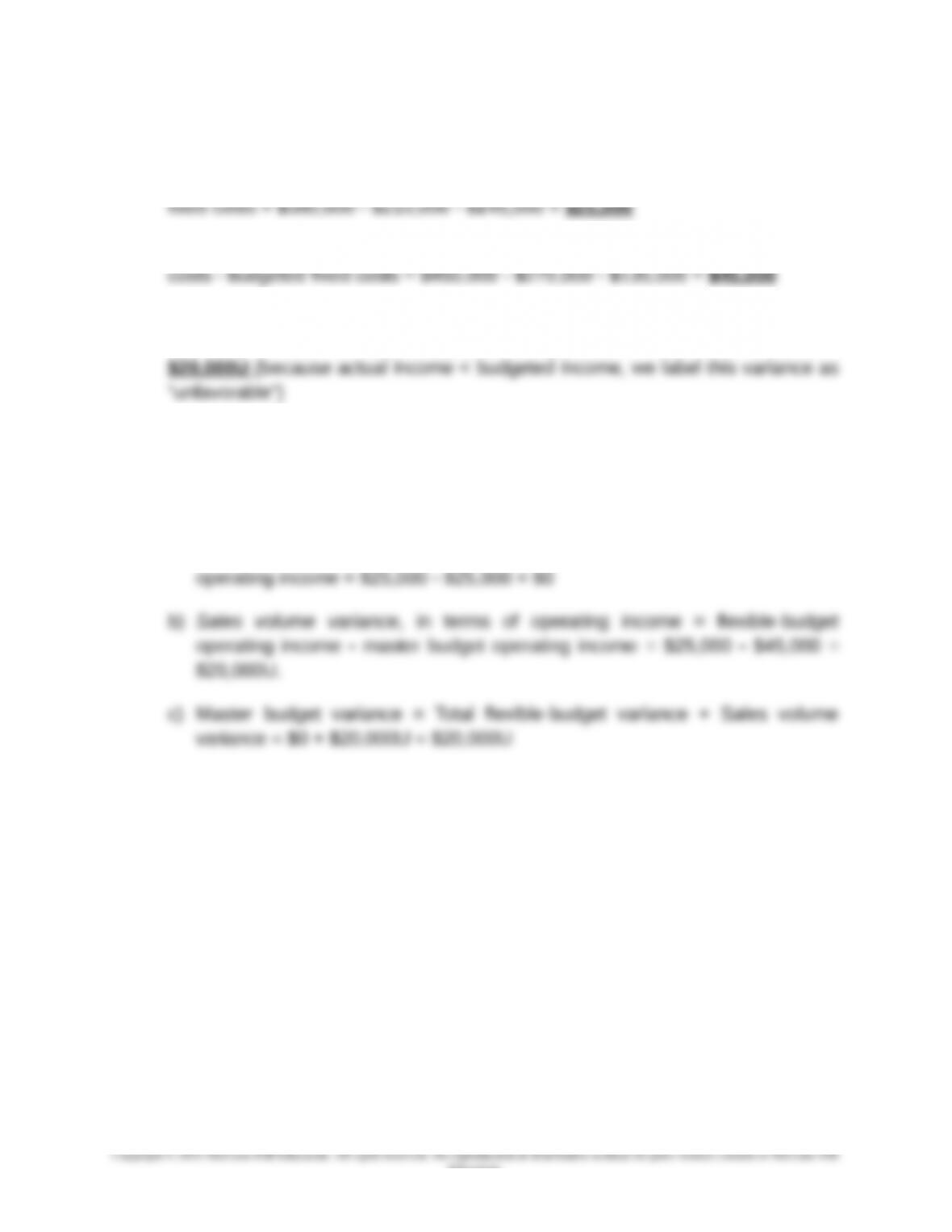
3. Total master (static) budget variance, in terms of operating income = actual
operating income master budget operating income = $25,000 $45,000 =
4. The first-level decomposition of the total master (static) budget variance in
operating income is accomplished through the introduction of a flexible-budget
(based on actual sales volume for the period). In this case, the flexible-budget
operating income = $400,000 $240,000 $135,000 = $25,000. Thus:
a) Total flexible-budget variance = actual operating income flexible-budget
14-11
Education.
Chapter 14 – Operational Performance Measurement: Sales, Direct-Cost Variances, and the Role of Nonfinancial
Performance Measures
14-24 (Continued)
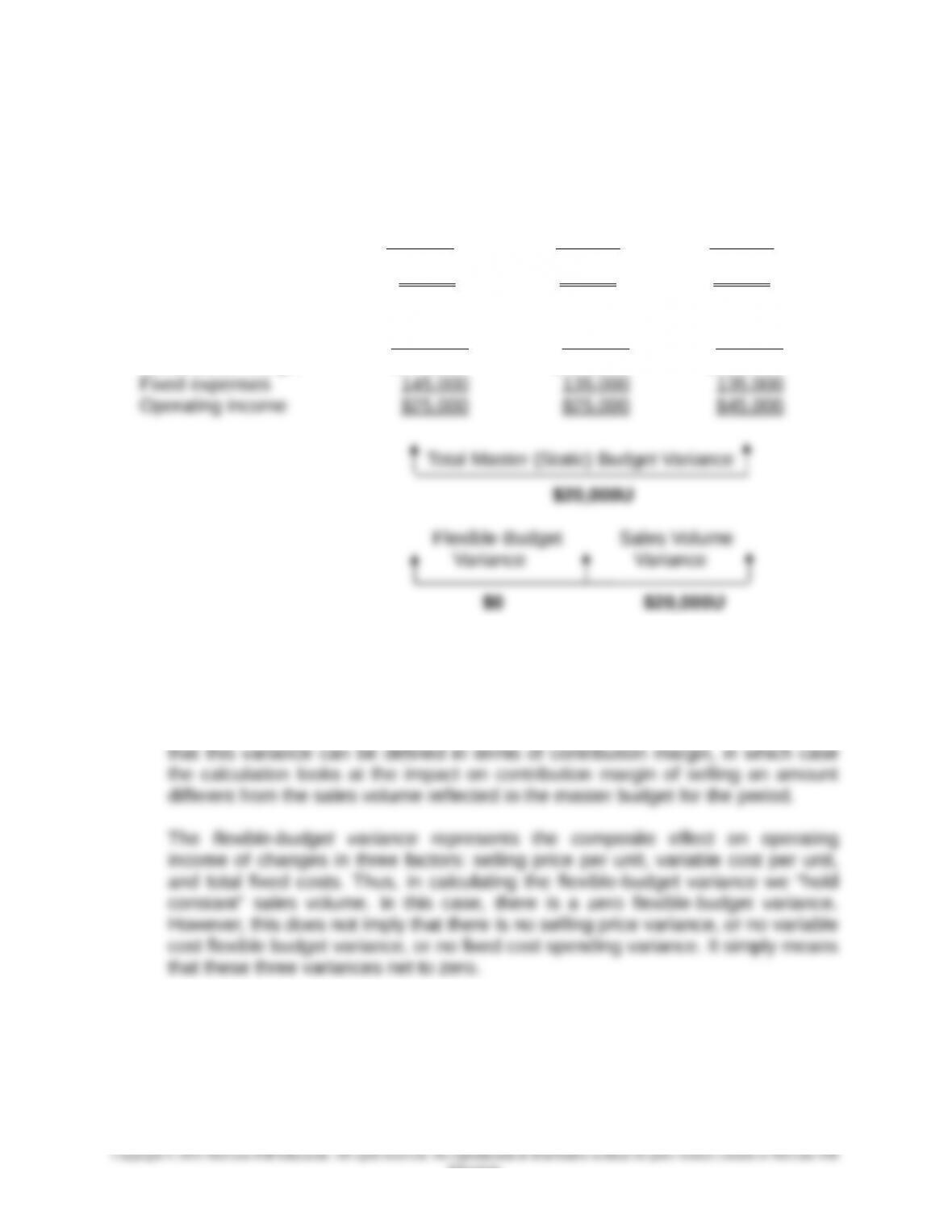
In tabular form, we have:
Actual Flexible Master
Results Budget Budget
Unit sales 40,000 40,000 45,000
Sales $380,000 $400,000 $450,000
Total variable expenses 210,000 240,000 270,000
Contribution margin $170,000 $160,000 $180,000
5. The sales volume variance represents the impact on operating profit of selling a
different volume of sales compared to the budgeted volume reflected in the
master budget. As such, the calculation of the variance holds three other factors
constant: selling price per unit, variable cost per unit, and total fixed costs. Note
14-12
Education.
Chapter 14 – Operational Performance Measurement: Sales, Direct-Cost Variances, and the Role of Nonfinancial
Performance Measures
14-25 Flexible Budget and Operating-Income Variances (45 minutes)
1. Flexible budget for June, based on 950 units produced/sold (95% of original master
budget):
Units sold 950
Sales (95% × $800,000) $760,000
Variable expenses (95% × $450,000) 427,500
2. Refer to text Exhibit 14.1 for master-budget data
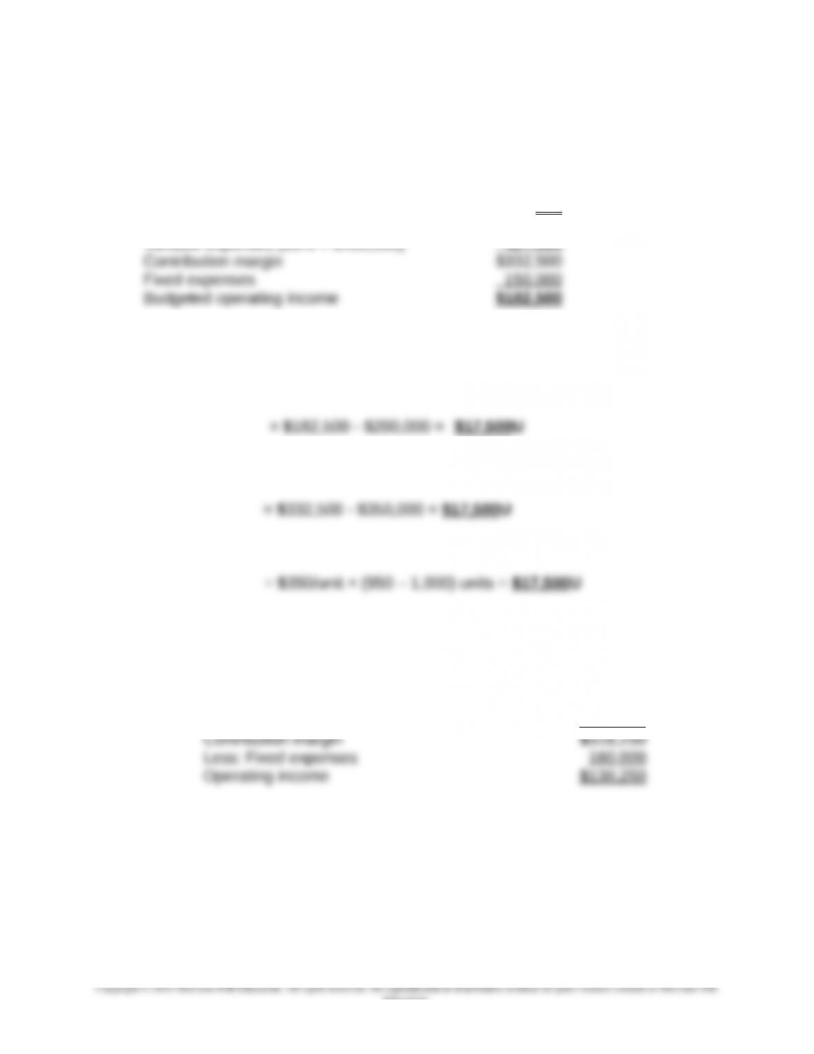
a. Sales volume variance, in terms of operating income = flexible-budget
operating income – master (static) budget operating income
b. Sales volume variance, in terms of contribution margin = flexible-budget
contribution margin master (static) budget contribution margin
or, budgeted cm/unit × (actual – master budget) sales volume
3.
Actual Operating Results
For the Month of June
Sales (950 units × $835/unit) $793,250
Less: Total variable expenses 475,000
14-13
Education.
Chapter 14 – Operational Performance Measurement: Sales, Direct-Cost Variances, and the Role of Nonfinancial
Performance Measures
14-25 (Continued)
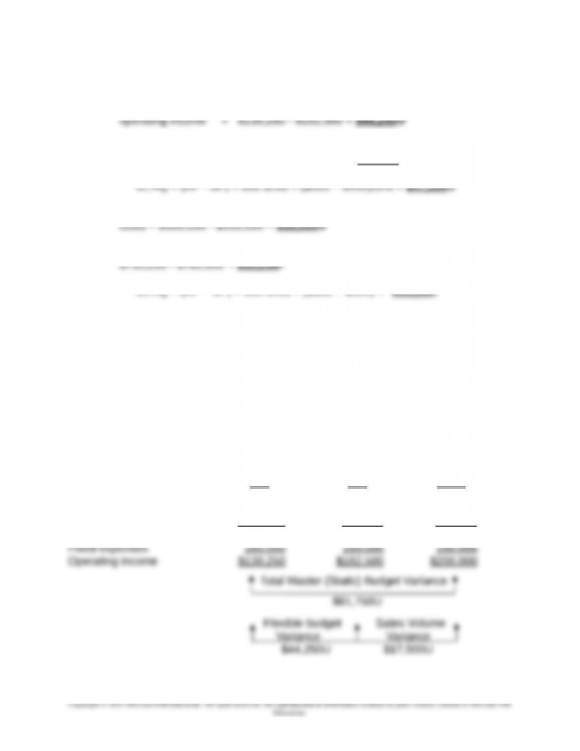
a. Total flexible-budget variance = actual operating income flexible-budget
b. Total variable cost flexible-budget variance = actual variable costs flexible-
budget variable costs = $475,000 $427,500 = $47,500U
c. Total fixed cost flexible-budget variance = actual fixed costs − flexible-budget fixed
d. Selling price variance = actual sales revenue − flexible-budget sales revenue =
or, AQ × (AP − SP) = 950 units × ($835 − $800) = $33,250F
NOTE: total flexible-budget variance ($44,250U) = selling price variance ($33,250F)
+ total variable cost flexible-budget variance ($47,500U) + total fixed cost flexible-
budget variance ($30,000U).
The following presentation, similar to text Exhibit 14.4, might be useful for in-class
presentation purposes:
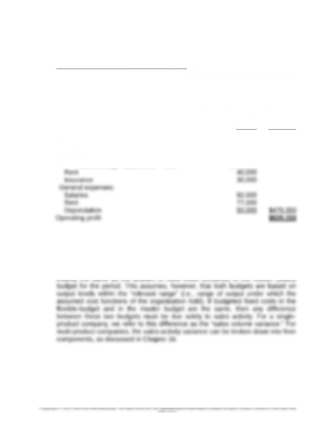
SCHMIDT MACHINERY COMPANY
Analysis of Operating Results
June 2016
Flexible Static (Master)
Actual Budget Budget
Unit sales 950 950 1,000
Sales $793,250 $760,000 $800,000
Total variable expenses 475,000 427,500 450,000
Contribution margin $318,250 $332,500 $350,000
14-14
Chapter 14 – Operational Performance Measurement: Sales, Direct-Cost Variances, and the Role of Nonfinancial
Performance Measures
14-26 Direct Materials and Direct Labor Variances (40 minutes)
Note: Refer to Exhibit 14.5 for standard cost information.
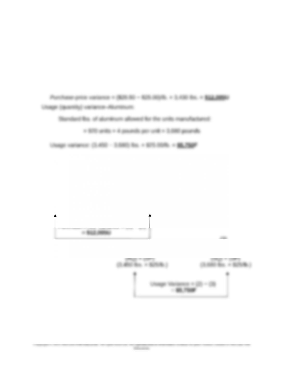
1. Purchase price variance–Aluminum:
Total lbs. aluminum purchased = lbs. used + ending inventory −
beginning inventory = 3,450 + 30 − 50 = 3,430 pounds
The following diagram, similar to text Exhibit 14.11, may be useful for in-class
presentation purposes.
(1) (2)
Actual Purchases Actual Purchases
at Actual Cost at Standard Cost
(AQ) × (AP) (AQ) × (SP)
(3,430 lbs. × $28.50/lb.) (3,430 lbs. × $25/lb.)
(3)
Actual Usage Flexible-Budget
at Standard Cost Amount
14-15
Chapter 14 – Operational Performance Measurement: Sales, Direct-Cost Variances, and the Role of Nonfinancial
Performance Measures
14-26 (Continued)
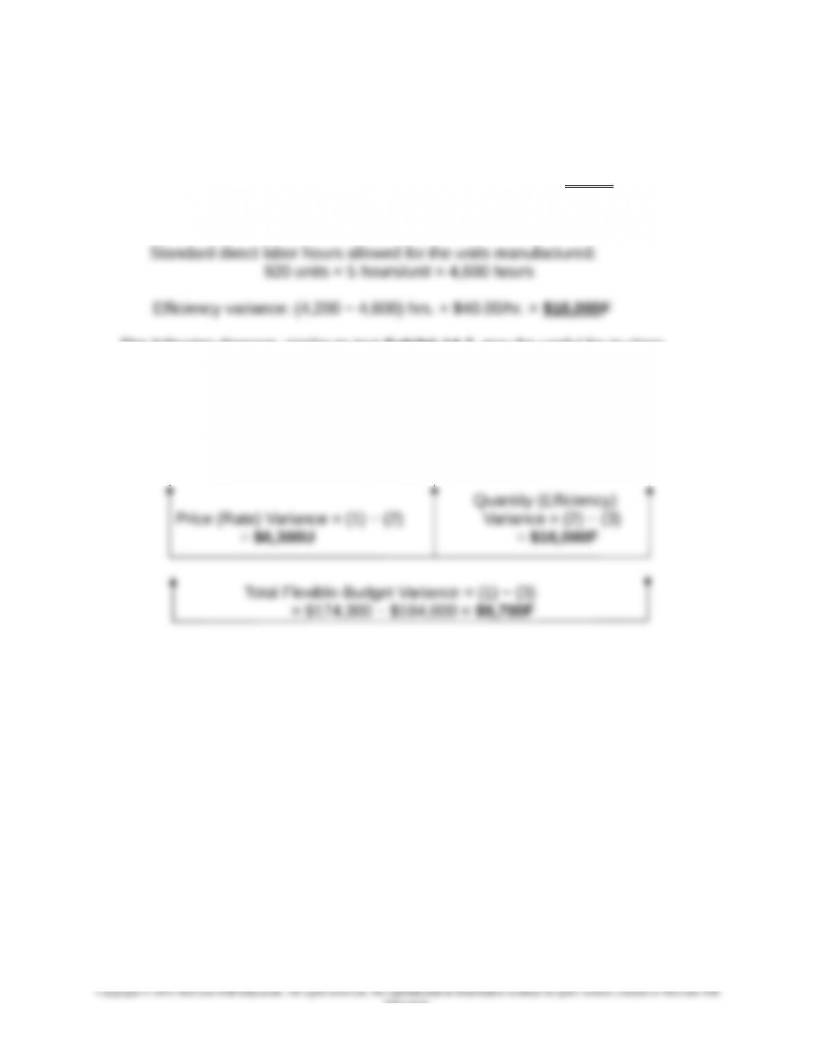
2. Direct labor rate variance: ($41.50 − $40.00)/hr. × 4,200 hrs. = $6,300U
Direct labor efficiency variance:
The following diagram, similar to text Exhibit 14.7, may be useful for in-class
presentation purposes:
(2) (3)
(1) Actual Input Flexible-budget
Actual Input Cost at Standard Cost Amount
(AQ) × (AP) (AQ) × (SP) (SQ) × (SP)
(4,200 hrs. × $41.50/hr.) (4,200 hrs. × $40/hr.) (4,600 hrs. × $40/hr.)
14-16
Education.
Chapter 14 – Operational Performance Measurement: Sales, Direct-Cost Variances, and the Role of Nonfinancial
Performance Measures
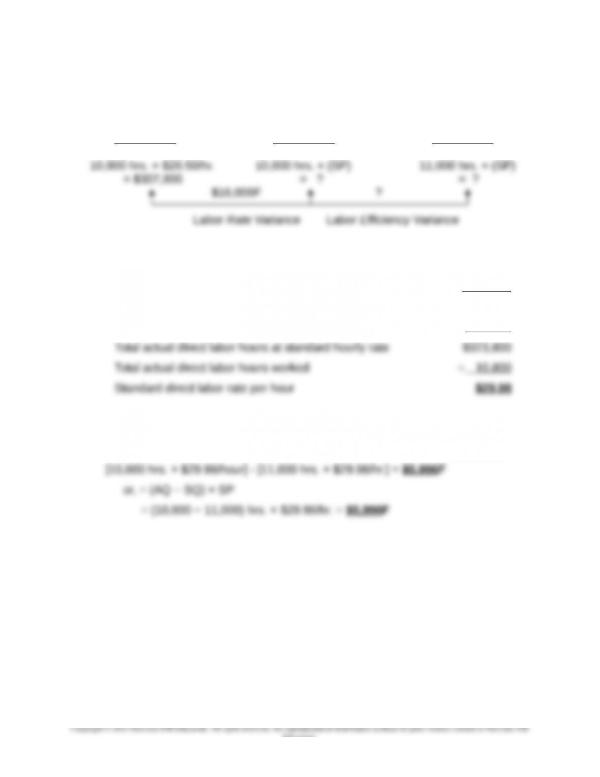
14-27 Standard Labor Rate and Labor Efficiency Variance (20 minutes)
Actual Inputs Actual Inputs Flexible-Budget
at Actual Cost at Standard Cost Amount
(AQ) × (AP) (AQ) × (SP) (SQ) × (SP)
1. Total actual direct labor hours worked 10,800
Actual hourly rate × $28.50
Total actual total direct labor cost $307,800
Plus: Favorable direct labor rate variance + 16,000
2. Direct labor efficiency variance = actual hours at standard cost standard labor
cost for units produced = [(AQ) × (SP)] [(SQ) × (SP)] =
14-17
Education.
Chapter 14 – Operational Performance Measurement: Sales, Direct-Cost Variances, and the Role of Nonfinancial
Performance Measures
14-28 Generating a Flexible Budget; Spreadsheet Application (50 minutes)
1. Flexible Budget, sales volume = 55,000 units
Sales (55,000 units × $31.00/unit) $1,705,000
Less: Cost of Goods Sold:
Direct materials (55,000 units × $2.80/unit) $154,000
Direct labor (55,000 units × $7.50/unit) 412,500
Manufacturing overhead:
Variable (40% × $412,500) 165,000
Fixed [$240,000 − (40% × $450,000)] 60,000 $791,500
Gross profit $913,500
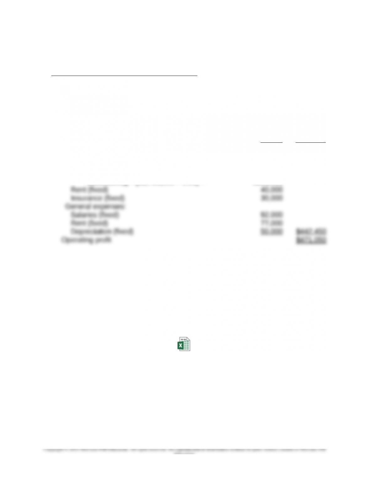
Less: Operating expenses:
Selling expenses:
Sales commissions [$1,705,000 × ($167,400
$1,860,000)] = [$1,705,000 × 0.09] = $153,450
Note to Instructor: An Excel file solution for Part 1 and Part 2 of Exercise 14-28 is
embedded below. You can open this “object” by doing the following:
1. Right click anywhere in the worksheet area below.
2. Select “worksheet object” and then select “Open.”
3. To return to the Word document, select “File” and then “Close and return
to…” while you are in the spreadsheet mode. The screen should then
return you to this Word document.
14-18
Education.
Ex. 14-28.xlsx
Chapter 14 – Operational Performance Measurement: Sales, Direct-Cost Variances, and the Role of Nonfinancial
Performance Measures
14-28 (Continued)
2. Flexible budget, sales volume = 65,000 units
Sales (65,000 units × $31.00/unit) $2,015,000
Less: Cost of Goods Sold:
Direct materials (65,000 units × $2.80/unit) $182,000
Direct labor (65,000 units × $7.50/unit) 487,500
Manufacturing overhead:
Variable (40% × $487,500) 195,000
Fixed [see answer, Part 1] 60,000 $924,500
Gross profit $1,090,500
Less: Operating expenses:
Selling expenses:
Sales commissions [$2,015,000 × ($167,400
$1,860,000)] = $2,015,000 × 0.09 = $181,350
3. The text uses the term pro-forma budget to refer to a budget prepared for any
level of operating activity for a given period. We reserve the term “flexible-budget”
to refer to the control budget prepared after the period based on the actual activity
level (e.g., sales volume) achieved. The flexible-budget is key to the financial
control process: it allows us to decompose overall variances into more detailed
components. Normally, the amount of fixed costs reported in the flexible-budget is
14-19
Education.
Chapter 14 – Operational Performance Measurement: Sales, Direct-Cost Variances, and the Role of Nonfinancial
Performance Measures
14-29 Behavioral Considerations and Continuous-Improvement Standards (25
minutes)
1. Direct labor hour standards and standard direct labor cost per unit, October –
January:
Month
Previous
Standard Reduction New Standard
Standard Direct
Labor Cost/Unit
October N/A N/A 1.50000 hr./unit $45.00
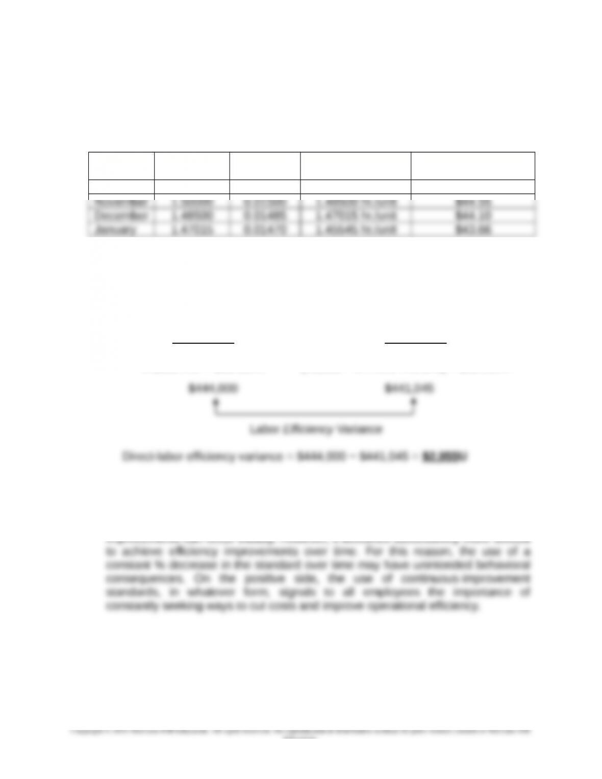
2. Computation of direct labor efficiency variance, December:
Actual Inputs Flexible-Budget
At Standard Cost Amount
(AQ) × (SP) (SQ) × (SP)
14,800 hrs. × $30.00/hr. (10,000 × 1.47015 hrs./unit) × $30.00/hr.
3. The basic trade-off is a problem similar to the situation with Kaizen: pushing
employees too hard for improvements, month after month. In response, workers
may perceive that the performance goal is simply not achievable, in which case
the standard itself loses its motivational value. In many processes, significant
14-20
Education.