
Chapter 14 – Operational Performance Measurement: Sales, Direct Cost Variances, and the Role of Nonfinancial
Performance Indicators
Chapter 14
Operational Performance Measurement: Sales, Direct Cost Variances, and the
Role of Nonfinancial Performance Indicators
Learning Objectives
LO 14-1 Explain the essence of control systems in general and operational control systems in
particular
LO 14-2 Explain the total operating-income variance for a given period
LO 14-3 Develop a general framework for subdividing the total operating-income variance into
component variances
LO 14-4 Develop standard costs for product costing, performance evaluation, and control
LO 14-5 Record manufacturing cost flows and associated variances in a standard cost system
LO 14-6 Discuss major operating functions and the need for nonfinancial performance indicators
New in this Edition
Revision of four end-of-chapter problems
Revision/updating of two Real-World Focus (RWF) items (Demystifying a Consumer Gas Utility
Bill, and Controlling Labor Costs through the Use of “Workforce-Management Systems”)
Four totally new Real-World Focus (RWF) items (Managing Health Care Costs through Use of
Standard Cost Information; Managing Supply-Chain Costs; Using Technology to Manage Energy
and Water Consumption; and the NFL Takes the Lead in Promoting Sustainability and
Environmental Responsibility)
Teaching Suggestions
This chapter and the next explain the role of standard costs, flexible budgets, and variances in the
planning and control of operations and in the assessment of short-run operating results. I usually begin
this chapter with an introduction to control systems in general and, more specifically, management
accounting and control systems, financial control, and operational control. Particular emphasis is placed
on the strategic role of standard costing: to motivate improvements in both operational effectiveness and
efficiency. I then introduce students to the notion of flexible versus master (static) budgets, which are key
components of a traditional financial control model. I explain how these tools can be used to explain why
actual and master budget operating income differed for a period. In other words, I begin with the notion
that, traditionally, such tools can be used to answer the following question: why did actual operating
income for the period just ended differ from the operating income contained in our master (static) budget?
This total difference, or variance, is referred to as the “total operating-income variance” for the period.
(This is also referred to as the “total static (master) budget variance for the period.”)
Thus, students learn the importance of flexible budgets and standard costs for operational and financial
control purposes, as part of an organization’s comprehensive management accounting and control system.
Before shifting to the calculations of direct cost variances, I discuss the determination of cost standards in
practice, taking into account the “new manufacturing environment” and using benchmarking and activity
analysis.
I often cover this chapter in two class meetings. In the first class I cover the determination of operating
income and contribution margin variances and the development of standard costs and variance analysis.
14-1
Education.
Chapter 14 – Operational Performance Measurement: Sales, Direct Cost Variances, and the Role of Nonfinancial
Performance Indicators
The general framework presented in the chapter is a particularly useful tool that allows students to
structure their analysis. Please see text Exhibit 14.2, Exhibit 14.4 and Exhibit 14.7 for general
guidelines.
On the second class-day I pick some longer problems and cover the limitations, behavioral and
implementation issues. For accounting majors I will also make sure the class understands the accounting
entries that accompany standard cost systems. Finally, as indicated by the revised title for this chapter, I
discuss the strategic role of nonfinancial information in a comprehensive management accounting and
control system. In this regard, we discuss basic business processes (such as operating processes) and the
limitations of traditional financial control mechanisms for helping to improve such processes. Special
attention can be given to Just-in-Time (JIT) manufacturing, as a strategic operating process choice, and
the need for both financial and nonfinancial performance indicators within this context. Finally, Exhibit
14.14 (Customer Response Time) and Process Cycle Efficiency (PCE) are introduced as specific
examples of nonfinancial performance indicators that are relevant to the control of a JIT system.
Assignment Matrix
End-of-Chapter Exercises & Problems
Chapter Learning Objectives
Text Features
7th
ed.
EOC
6th
ed.
EOC
Transition
6e to 7e
X = included in Connect
Est.
Time
1. Essence of Ctl. systems
2. Explain total operating- income variance
3. Component Variances
4. Standard setting
5. Journal entries
6. Operating Functions/ Nonfinancial Indicators
Service
Ethics
Brief Exercises
14-13
14-14
Revised
X
5 min
X
14-14
14-17
–
X
10 min
X
X
14-15
14-13
–
X
5 min
X
14-16
14-16
–
X
5 min
X
14-17
14-15
–
X
5 min
X
14-18
14-18
Revised
X
5 min
X
14-19
14-19
Revised
X
5 min
X
14-20
14-20
Revised
X
5 min
X
14-21
14-21
Revised
X
5 min
X
14-22
14-22
Revised
X
5 min
X
Exercises
14-23
14-26
–
X
50 min
X
X
X
14-24
14-27
–
X
45 min
X
X
14-25
14-28
–
X
45 min
X
X
14-26
14-29
–
X
30 min
X
14-27
14-30
–
X
20 min
X
14-28
14-31
–
X
50 min
X
14-29
14-32
Revised
X
25 min
X
X
14-30
14-33
Revised
X
45 min
X
X
14-31
14-34
–
–
40 min
X
X
14-32
14-35
–
X
15 min
X
Continued on next page …
Chapter 14 Assignment Matrix—Continued
End-of-Chapter Assignments
Chapter Learning Objectives
Text Features
14-2
Education.
Chapter 14 – Operational Performance Measurement: Sales, Direct Cost Variances, and the Role of Nonfinancial
Performance Indicators
7th
ed.
EOC
6th
ed.
EOC
Transition
6e to 7e
X = included in Connect
Est.
Time
1. Essence of Ctl. systems
2. Explain total operating- income variance
3. Component Variances
4. Standard setting
5. Journal entries
6. Operating Functions/ Nonfinancial Indicators
Strategy
Service
International
Ethics
Sustainability
14-33
14-36
–
–
25 min
X
X
14-34
14-37
–
–
15 min
X
X
14-35
14-23
–
–
20 min
X
X
14-36
14-38
–
X
15 min
X
14-37
14-40
Revised
X
40 min
X
X
14-38
14-39
–
X
30 min
X
X
14-39
14-24
–
–
15 min
X
X
14-40
14-25
–
–
45 min
X
X
X
X
14-41
14-41
–
–
45 min
X
X
14-42
14-42
–
X
45 min
X
X
X
Problems
14-43
14-43
–
–
90 min
X
X
14-44
14-44
Revised
–
25 min
X
X
14-45
14-45
Revised
–
35 min
X
14-46
14-46
Revised
–
45 min
X
X
X
14-47
14-47
–
–
45 min
X
14-48
14-48
–
–
60 min
X
X
14-49
14-49
Revised
–
60 min
X
X
X
X
14-50
14-50
–
–
50 min
X
X
X
X
14-51
14-51
Revised
–
75 min
X
X
X
X
X
14-52
14-53
–
–
30 min
X
X
X
X
14-53
14-54
–
–
60 min
X
X
X
X
14-54
14-55
–
–
40 min
X
X
X
X
–
14-52
Deleted
Lecture Notes
Management Accounting and Control Systems (MACS): I generally start this chapter with a
discussion of the following elements, which are each part of an organization’s comprehensive
management accounting and control system (MACS):
Operational control (i.e., control of major operational processes)
Financial control:
Master budget
Flexible budget
Standard costs
Variances
Variances
A variance is the difference between an actual operating result and a budgeted or standard amount for the
operation. Variances are labeled as favorable or unfavorable. A favorable variance (F) has the effect of
14-3
Education.

Chapter 14 – Operational Performance Measurement: Sales, Direct Cost Variances, and the Role of Nonfinancial
Performance Indicators
increasing short-run operating profit while an unfavorable variance (U) has the effect of decreasing
short-run operating profit. Various revenue and cost variances are key outputs of a traditional financial
control system used to explain the total operating-income variance for the period, as explained more fully
below.
Total Operating-Income Variance = Static Budget Variance = Master Budget Variance
An indication of the financial effectiveness of operations during the period is the total operating
income variance, which defined as the difference between actual operating income for the period and the
amount of operating income reflected in the master (static) budget for the period. See text Exhibit 14.1.
Master (Static)
Actual Operating Income Budget Operating Income
Total Operating-Income Variance
I generally tell students that short-term operating profit is a function of five factors: selling price per unit,
variable cost per unit, total fixed costs, sales volume (quantity), and sales mix. If we assume a single-
product context, then any operating-income variance for the period should be explainable by the other
four factors being different from plans. The process of explaining the total operating income variance is
referred to as “variance decomposition.” Exhibit 14.2 can be used to provide students with the “big
picture” of variance analysis.
Flexible Budget Variance and Sales Volume Variance
The key to the decomposition of the total operating-income variance for a period is the introduction of a
flexible budget (FB) based on outputs (i.e., on actual unit sales). A first-level decomposition of the
“operating income variance” for a single-product firm results in a total flexible budget (FB) variance
and a sales volume variance. See text Exhibit 14.4.
A flexible budget (FB) based on output is developed using budgeted selling price per unit, budgeted
(standard) direct costs per unit, and budgeted total fixed costs for the actual output level achieved during
the period. Once this FB is determined, a first-level decomposition of the total operating income variance
can be performed. The sales volume variance is the difference between the master budget and the
flexible budget (FB) based on output. It measures the effects of changes in output on sale revenues,
expenses, contribution margins, and operating income. The total flexible-budget variance is the
difference between actual operating income of the period and the flexible budget based on output. It
measures the effects of efficiencies in using resources on expenses, contribution margins, and operating
income and the effects of changes in selling prices of output units on sales revenues and subsequent
effects on contribution margin and operating income. Together, the sales volume variance + the total
flexible budget variance = total operating income variance, as indicated below:
Actual Operating Flexible Budget Master
Income Based on Output (Static) Budget
Total Flexible-Budget Variance Sales Volume Variance
Standard Costs and Input Quantities
A standard cost is a measure of the cost that should be incurred to manufacture a product or provide a
service. Establishing a standard requires careful analysis of operations. A standard can be an ideal
standard or a currently attainable standard. An ideal standard demands perfect implementation and
14-4

Chapter 14 – Operational Performance Measurement: Sales, Direct Cost Variances, and the Role of Nonfinancial
Performance Indicators
maximum efficiency in every aspect of the operation and is not easily attainable. A currently attainable
standard sets the performance criterion at a level that workers with proper training and experience can
attain most of the time without extraordinary effort. An example of a standard cost sheet is provided in
Exhibit 14.5.
A firm can use activity analysis, historical data, benchmarks, market expectation, target cost, or strategic
decision to set the standards. Setting the standard using activity analyses requires analyses of all activities
required to complete a job, project, or operation. It is often expensive and time-consuming.
Benchmarking is the process of measuring products, services, and activities against the best performance.
Using benchmarking to set standard has the advantage of using the best performance anywhere as the
standard and help the firm to maintain its competitive edge. The target cost for a product is the cost that
will yield the desired profit margin, given the market price of the product.
The availability of standard cost (and revenue) information enables the managerial accountant to
breakdown the total flexible budget variance into its components: a total selling price variance and a
flexible budget variance for each cost, variable and fixed. The fixed cost variances are called “spending
variances.”
Further decomposition of the fixed cost variances would be to assign each spending variance to a
responsibility center (product, department, geographic region, manager, etc.). The series of variable cost
flexible budget variances can each be broken down into price (p) and quantity/efficiency (q) components,
as discussed below for direct labor and direct materials.
Direct Cost Variances: Materials and Labor
A manufacturing firm usually has a standard cost sheet that details the standard quantity and standard cost
for all the significant cost elements of the operations. Typical standards include standards for direct
materials (DM) and direct labor (DL). A DM flexible budget variance can be separated, for each material,
into a DM price and a DM usage variance. A DL flexible budget variance can be further divided into DL
rate and DL efficiency variances, by developing a second flexible budget, that is, one based on actual
resource inputs (actual units of material or actual labor hours worked). A diagrammatic representation of
the variance decomposition process for DM and DL costs follows (see Exhibit 14.7, Exhibit 14.8,
Exhibit 14.9, and Exhibit 14.10):
Direct Materials Variances
FB Based on Output
Actual FB Based on Inputs (Standard Quantity of DM Allowed for
Cost Incurred (Quantity Used × Standard Cost) Output Achieved × Standard Cost)
(AQ × AP) (AQ × SP) (SQ × SP)
Price Variance Usage Variance1
NOTE: If the company calculates the DM price variance at point of purchase, this variance is referred to
as the direct materials purchase price variance. When this is the case, then AQ in the price variance
formula refers to the Actual Quantity purchased. For the usage (efficiency) variance calculation, AQ
stands for Actual Quantity issued to (consumed in) production.
If the price variance for materials is not calculated until the materials are issued to production, then AQ in
the above diagram stands in all cases for Actual Quantity used (issued to production) during the period.
1 If there are multiple labor classes (categories) that are substitutable, then it is possible to break the direct labor
efficiency (quantity) variance into a direct labor mix variance and a direct labor mix variance. As noted below, if
there are multiple direct materials, and these materials are substitutable, then the direct materials quantity variance
can similarly be broken down into a mix variance and a yield variance.
14-5
Education.

Chapter 14 – Operational Performance Measurement: Sales, Direct Cost Variances, and the Role of Nonfinancial
Performance Indicators
Direct Labor Variances
FB Based on Output
Actual FB Based on Inputs (Standard DLHs Allowed for the
Cost Incurred Actual Hours x Standard Hourly Rate Output x Standard Hourly Rate)
(AH × AR) (AH × SR) (SH × SR)
Rate Variance Efficiency Variance
Standard Setting
At this point, the instructor can provide a more detailed explanation of the standard-setting process—that
is, the choices that need to be made and the technical details regarding standard costs.
Cost and Asset Flows and Journal Entries
I find it helpful to start this material with a discussion of the difference between standard costs and the use
of a standard cost system. I then transition to a discussion of the “big picture” or framework presented as
Exhibit 14.12.
For companies using a standard cost system and recognizing the materials price variance at point of
purchase, the raw materials inventory account debited (charged) for materials purchased during the
period. Any difference between the standard cost of items purchased and the actual price paid is recorded
in a separate “materials purchase price variance” account. Standard usage of raw materials (based on
output produced) at standard cost is charged to the Work-in-Process (WIP) Inventory account. Any
difference is charged to the “materials usage variance” account.
Direct labor is also charged to production (work in process) at standard rates for the standard allowed
hours for the units manufactured. The effect of paying a non-standard wage rate for the period is recorded
in a separate “direct labor rate variance” account while the effect of using a non-standard amount of labor
hours to produce the current period’s output is recorded in a separate “direct labor efficiency variance”
account.
The standard cost of units completed is transferred from the WIP Inventory account to the Finished Goods
Inventory account. Units sold are cleared from the Finished Goods Inventory account and charged to Cost
of Goods Sold (CGS)–again at standard manufacturing cost.
For those instructors covering journal entries, the discussion can conclude with an examination of the T–
accounts presented in Exhibit 14.13.
Limitations of Standard Costing and Short-Term Financial Performance Indicators
Standard cost variances are often reported to managers too late for them to take timely corrective
action.
Direct Labor (DL) has become less significant and tends to be more fixed than variable. A focus
on labor efficiency variances tends to encourage production of excess inventories (counter to, say,
a JIT philosophy).
A key objective in the new manufacturing environment is to increase quality. An overemphasis on
cost may result in lower quality. For example, focusing on the materials price variance may result
in the purchase of low quality materials.
14-6
Chapter 14 – Operational Performance Measurement: Sales, Direct Cost Variances, and the Role of Nonfinancial
Performance Indicators
Competitive conditions often require continuous improvement; attaining preset standards isn’t
sufficient.
The need to identify basic business processes and how such processes are most effectively
“controlled.”
Nonfinancial performance indicators are needed to supplement financial performance indicators.
The move to JIT can be used as a specific example of an operating process decision. Associated
with this process is the need to monitor and report key performance indicators, such as Customer
Response Time (CRT) and Process Cycle Efficiency (PCE), both of which are nonfinancial in
nature but strategically important from a control/performance reporting perspective.
Breakdown of Material and Labor Quantity (Efficiency) Variance
As noted above, if resource inputs (labor and materials) are substitutable, then cost efficiencies can be
achieved either by (1) using a less expensive mix of materials to produce a given level of output, or (2)
using less material (in total) to achieve that level of output. These two elements refer, respectively, to the
materials mix variance and the materials yield variance. When added together, these two variances equal
the sum of efficiency (usage) variance for all direct materials, calculated individually using the procedure
depicted in Exhibit 14.9. To break down the total materials quantity (usage) variance into mix and yield
components, we expand Exhibit 14.9 as follows:
1. The exhibit must be expanded to include (in a single exhibit) all substitutable materials
2. Existing column (2) is expanded to represent, for each direct material, the product of the actual
3. Existing column (3) is expanded to represent, for each direct material, the product of the standard
total quantity of all direct materials that should have been used during the period by the standard
input mix percentage for the direct material and by the standard cost per unit of the material
The difference between the total of column (2) and column (3) is the total materials usage (quantity)
variance. This variance can be broken down by inserting a new column (call it 2’) between the two, as
follows:
For each direct material, take the product of the actual total quantity of all direct materials used
during the period (same number used in revised column 2) multiplied by the standard input mix
percentage for the direct material and by the standard cost per unit of the material.
The difference between the total of column 2 and the total of column 3 is the total materials usage
(quantity) variance for the period. The difference between column and column 2’ is the materials mix
variance, while the difference between column 2’ and column 3 is the materials yield variance.
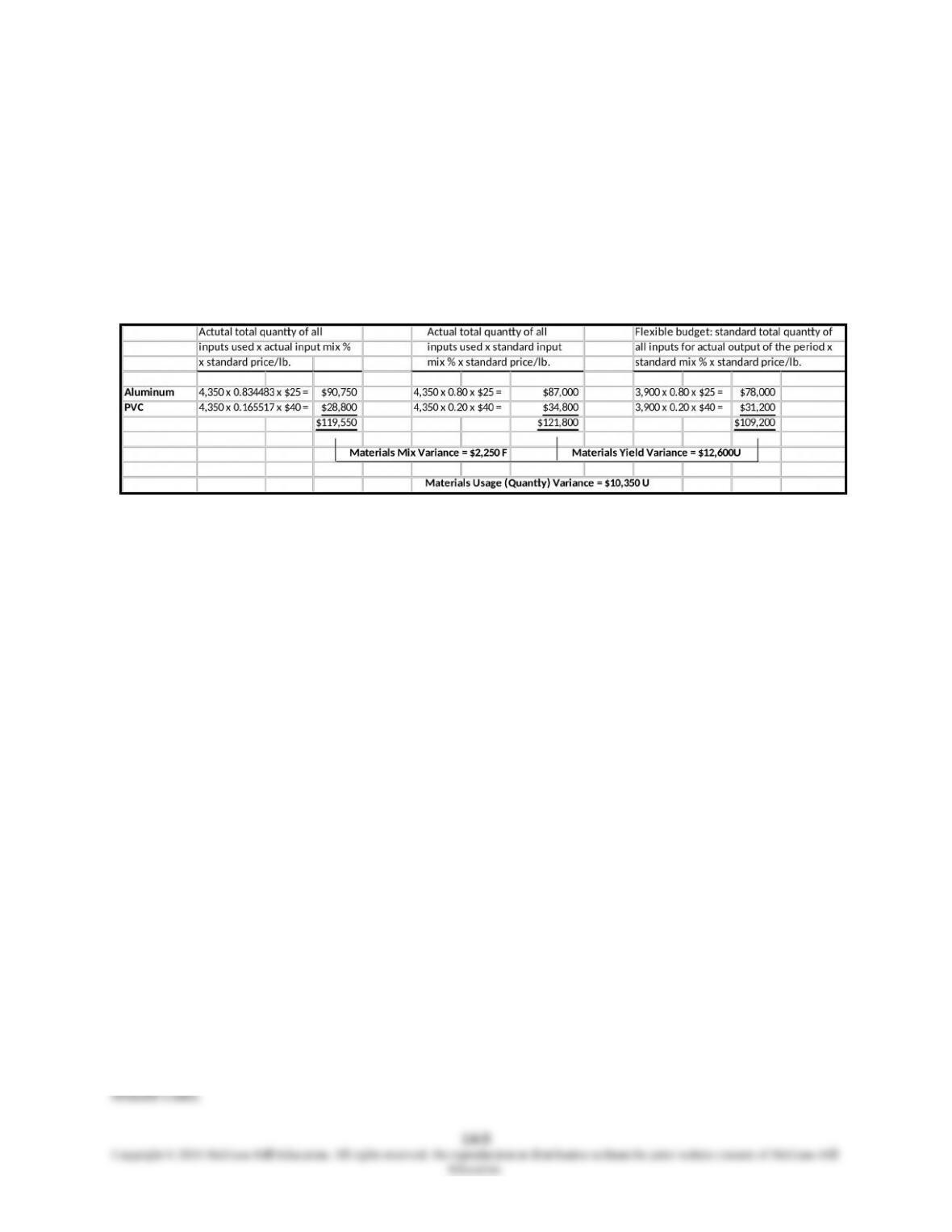
Example: Consider, for example, the direct materials information presented in text Exhibit 14.8. Assume
that management of Schmidt Machinery Company has some latitude in substituting aluminum and PVC.
As indicated in Exhibit 14.5, the standard mix of aluminum to PVC is 4:1 (i.e., 80%:20%). In Exhibit
14.8 we see that during October the actual direct materials mix was 83.4483%:16.5517% (i.e., 3,630
pounds:720 pounds). Total actual pounds of direct materials used = 3,630 + 720 = 4,350. Actual units
produced in October = 780. Total direct material units that should have been used (at standard) to produce
780 units = 5 lbs./unit x 780 units = 3,900 lbs.
14-7
Chapter 14 – Operational Performance Measurement: Sales, Direct Cost Variances, and the Role of Nonfinancial
Performance Indicators
As shown by the calculations below, the total direct materials usage (quantity) variance for October was
$10,350U. This total variance is explained by a favorable mix variance ($2,250) and an unfavorable yield
variance ($12,600). The mix variance is favorable because the units produced this period (780) used a
greater percentage of the less expensive raw material, aluminum. On the other hand, this shift to the
lower-cost material seems to have required total direct material inputs (4,350 lbs.) much higher than
should have been the case (3,900 lbs.).
Schmidt Machinery Company
October 2016
Materials Usage Variance and Breakdown into Mix and Yield Components
Economic Order Quantity (EOQ)
In most cases, students cover this material in an operations management (or, production & operations
management) class they take as part of the requirements for an accounting major. This is not universal,
however. Therefore, in the space below we present a discussion of EOQ, which the instructor can choose
to use in conjunction with Chapter 14.
As implied by its name, the EOQ model specifies the optimal order size, based on two key assumptions:
1. Demand for (and therefore use of) items ordered is fairly uniform throughout the year
2. Each new order is delivered in full when the inventory level reaches zero
In the basic EOQ model, total annual cost of stocking a given inventory item is equal to the sum of the
total purchase price of the item, plus the cost of ordering (assumed a batch-level cost, that is, fixed in
terms of order size), plus the cost of holding (carrying) the item in inventory. If we let D = annual demand
for the item, C = purchase price per unit, S = cost of placing an order, i = the cost of holding one unit in
inventory for one year (expressed as a percentage of C), and Q = order size (i.e., amount ordered each
time an order is placed), then the total annual cost of inventory (including cost of the item, holding costs,
plus ordering costs) can be written as:
TC = DC + (D/Q)S + (Q/2)Ci
Figure A below depicts, for a hypothetical example, alternative ordering strategies (order sizes) and the
resulting impact on total inventory-related cost (TC) as well as component costs, (D/Q)S and (Q/2)Ci
(with assumed uniform inventory usage, the average inventory held during a period = Q/2). Thus, the key
issue is determining the optimal order size for the inventory item in question. Note that as the order size
increases, annual ordering costs ((D/Q)S) decrease while annual holding costs ((Q/2)Ci) increase. The
goal is to minimize TC, that is, the goal is to choose an order size (Q) that minimizes total inventory-
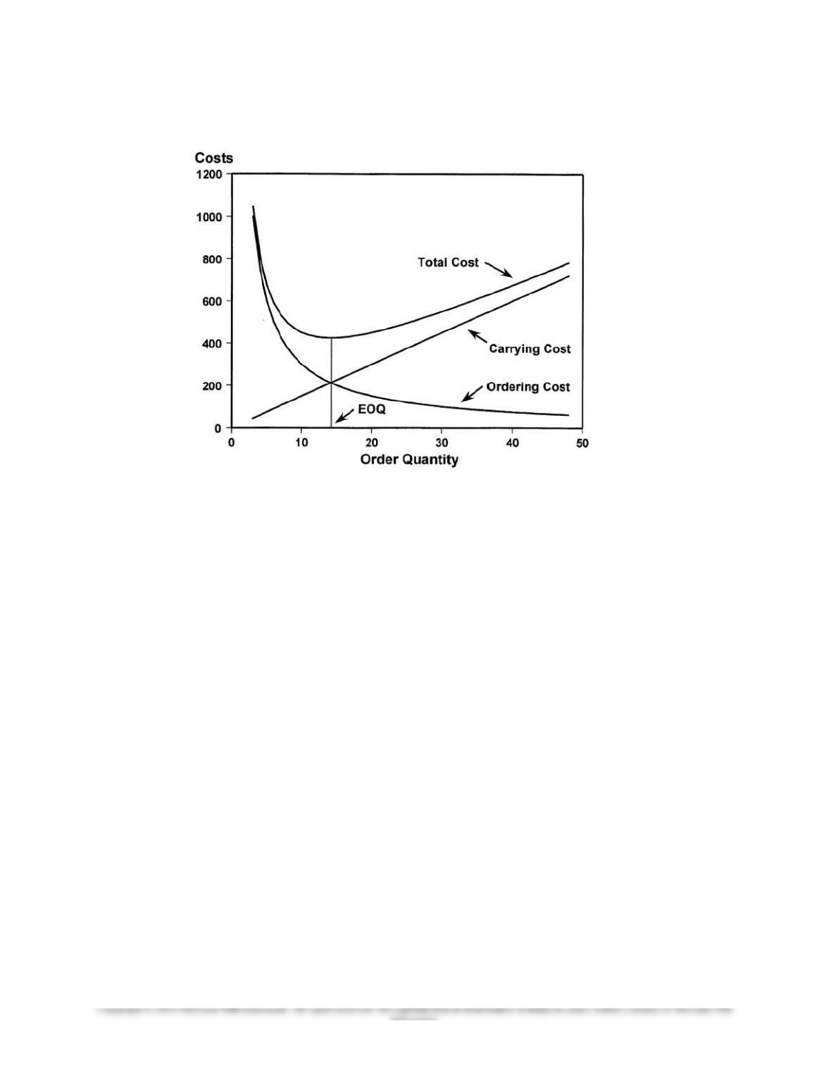
Chapter 14 – Operational Performance Measurement: Sales, Direct Cost Variances, and the Role of Nonfinancial
Performance Indicators
Figure A: Relationship between Order Size (Quantity), Annual Carrying Cost, Annual Ordering
Cost, and Total Inventory-Related Cost
One approach to determining the optimal order size (EOQ) is to use the Solver routine in Excel (note,
however, that because the underlying model—as shown above in Figure A—is nonlinear, you should not
chose Linear optimization under Solver). As depicted in Figure A, EOQ (given the preceding
assumptions) will occur when Inventory Carrying Costs and Inventory Holding Costs are in balance (15
units in the given example).
For a concrete example of determining EOQ, assume the following:
D = 24,000 units (annual demand)
C = $35 per unit (inventory purchase price)
S = $50 (the cost of placing an order)
i = 18% (inventory holding cost, expressed as a percentage of inventory cost)
Using Solver, we find that EOQ = 617.21 units. This would result in a total purchase cost of $840,000
(24,000 × $35/unit), annual ordering cost of $1,944, and an annual inventory holding cost of $1,944. Total
Cost (TC) under this ordering plan = $843,888.
As an alternative to using the Solver routine in Excel, we could use the following formula to determine
the EOQ:
In the preceding example, we have the following inputs:
2DS = 2 × 24,000 × $50 = $2,400,000
Ci = $35/unit × 0.18 = $6.3
14-9
Education.

Chapter 14 – Operational Performance Measurement: Sales, Direct Cost Variances, and the Role of Nonfinancial
Performance Indicators
Thus,
EOQ = = 617.214
Finally, it is worth emphasizing to students that the basic EOQ model can be extended to address
important “real-world” extensions, such as the existence of quantity discounts or storage space (or
financial) restrictions that might exist.
14-10
Education.