978-0077733773 Chapter 11 Solution Manual Part 8

Unlock access to all the studying documents.

View Full Document

11-46 (Continued-1)

$4.000 $27,435 $27,389

$4.250 $28,087 $27,944

$4.500 $28,739 $28,500

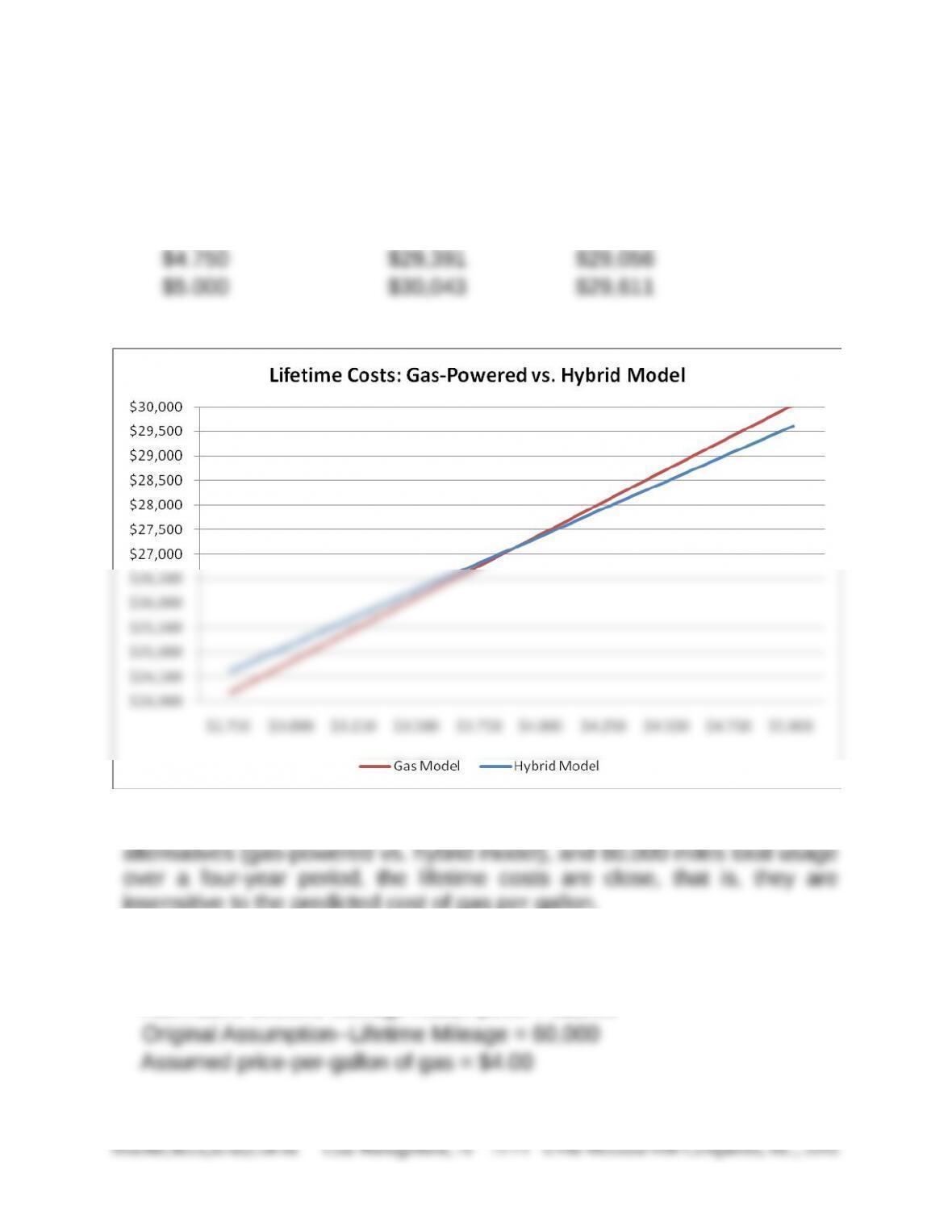
Based on the above analysis and graph, we see that for these two

insensitive to the predicted cost of gas per gallon.

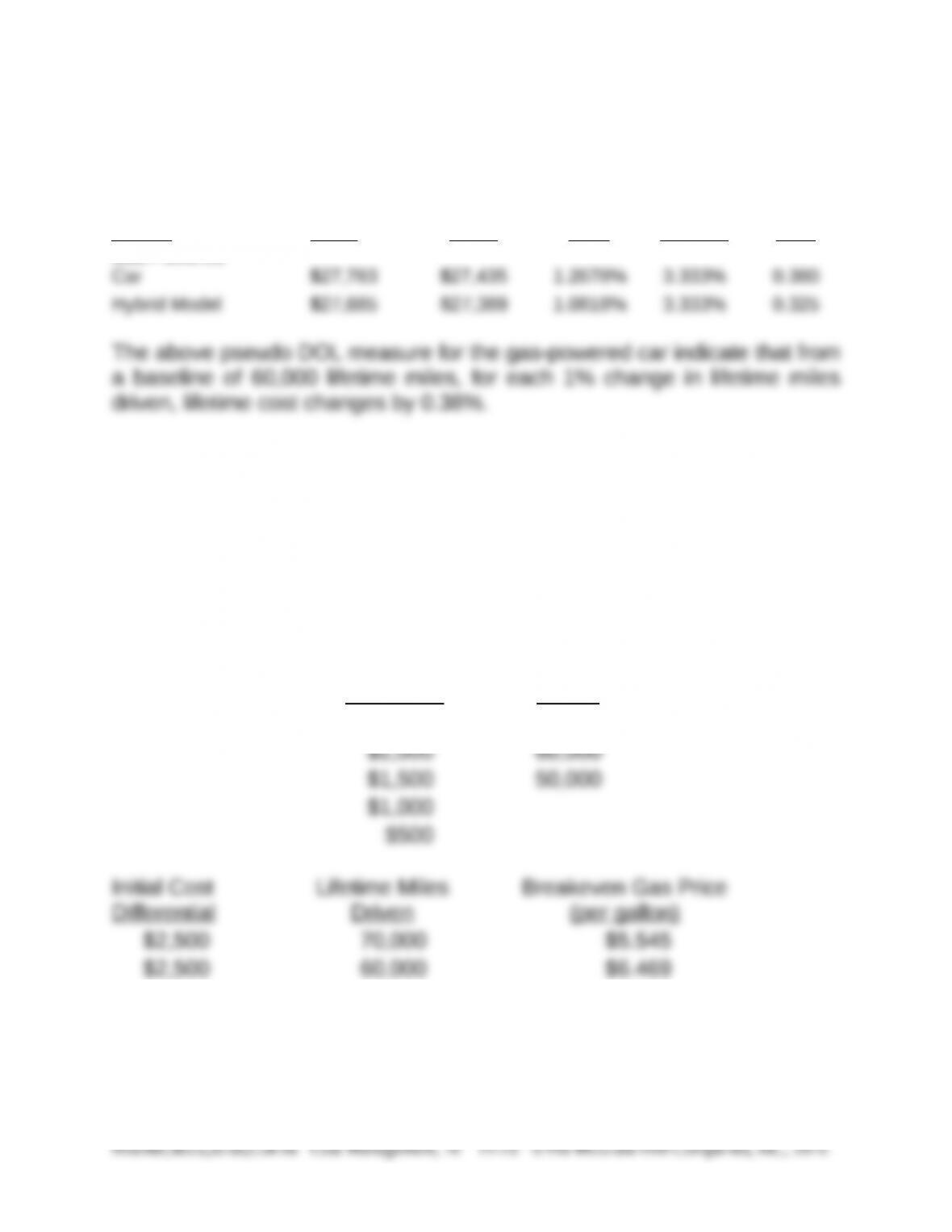
4. Pseudo degree of operating leverage (DOL) measure

Alternative Lifetime Mileage Assumption = 62,000

11-42 (Continued-2)

Lifetime Cost Lifetime Cost %

Option

@ 62,000

miles

@ 60,000

miles

Change

Cost

% Change

Mileage

Pseudo

DOL

Gas Powered

The relevant measure for the hybrid, from this base, is 0.325%. What this

tells us is that for this particular example, lifetime cost for both decision

alternatives is approximately equally sensitive to changes in lifetime miles

driven.

5. Decision Table–Break-even gas price as a function of different

combinations of initial cost differential (Hybrid cost [net of rebate] −

Cost of gasoline-powered model) and lifetime miles driven

Initial Cost

Difference

Lifetime Miles

Driven

$2,500 70,000

11-42 (continued-3)

Blocher,Stout,Juras,Cokins Cost Management, 7e 11-72 ©The McGraw-Hill Companies, Inc., 2016

Initial Cost

Differential

Lifetime Miles

Driven

Breakeven Gas Price

(per gallon)

$2,500 70,000 $5.545

$2,500 60,000 $6.469

$2,500 50,000 $7.763

$2,000 70,000 $4.436

$2,000 60,000 $5.175

$2,000 50,000 $6.210

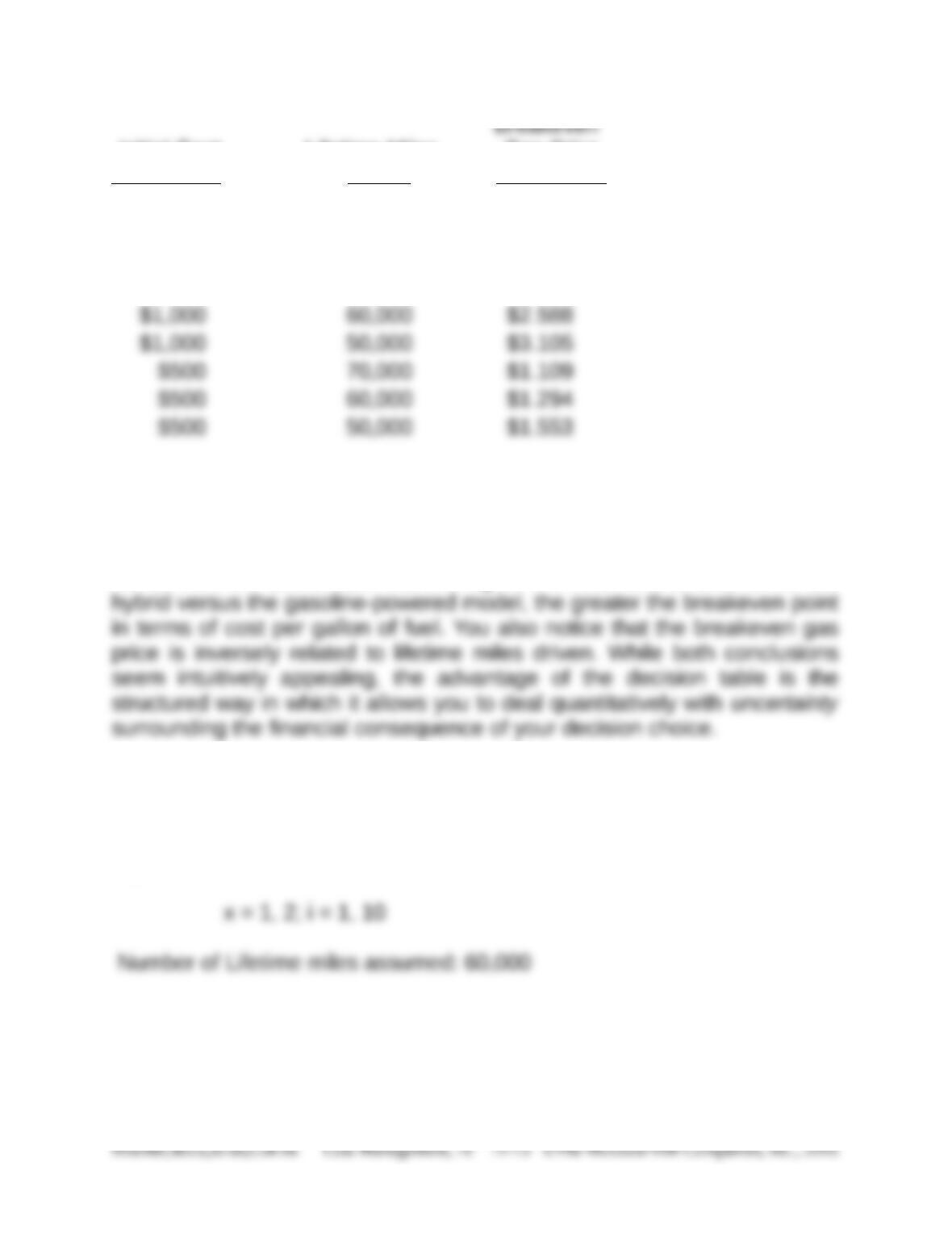
Initial Cost Lifetime Miles Gas Price

Differential Driven (per gallon)

$1,500 70,000 $3.327

$1,500 60,000 $3.881

$1,500 50,000 $4.658

$1,000 70,000 $2.218

For example, for the base case ($1,500 initial cost difference and 60,000

lifetime miles driven) the breakeven price per gallon is $3.881 (as found

earlier in part 2). At this price, and all other things equal, you would be

indifferent between the hybrid model and the gasoline-powered model.

Notice from the above table that the higher the initial cost differential for the

6. Expected value calculations:

E(ax) = ∑(Lifetime costi × pi)

i=1

9-42 (continued-4)

Action (Decision)

i Event p Hybrid Gas Model

1 $2.75 0.01 $246 $242

2 $3.00 0.05 $1,258 $1,241

3 $3.25 0.05 $1,286 $1,274

4 $3.50 0.05 $1,314 $1,307

5 $3.75 0.15 $4,025 $4,017

6 $3.88 0.15 $4,069 $4,069

Lifetime cost = initial cost outlay (F) + variable (gas) cost over four-year

period

Example: for the hybrid model, if the probability of gas selling at

$2.75/gallon is 0.01, then the appropriate amount is cost

component for calculating expected lifetime cost is:

To minimize the expected lifetime cost, we should choose the hybrid

model. However, these expected values are so close that they are

effectively equal, particularly given uncertainty in the price of gas. Thus, if

total miles driven over the lifetime of each vehicle (4 years) is 60,000,

then the expected lifetime cost of both actions (given the assumed

probability distribution) is approximately equal.

Finally, note that basing the decision solely on expected value (in the

present case, cost) ignores the risk preferences (utility function) of the

decision-maker. The decision table presented above in part 5 can

facilitate this discussion.

11-42 (continued-5)

7. Student answers will likely differ. Below are representative considerations.

Qualitative Considerations

a. safety record–does this differ between the two models?

b. reliability–does this differ between the two models? (in some cases, the

reliability of new models is considerably less than the reliability of older,

more established models)

c. as noted in conjunction with the discussion of decision tables (above),

we have not given explicit consideration to the decision-maker’s

attitude toward risk associated with the inputs to the decision model

d. “carbon footprint” issue–it is true that from an operating standpoint, the

carbon footprint of the hybrid would be less than it is for the related

gasoline-powered model. However, what this comparison ignores is the

total carbon footprint–from manufacture, through use (operation),

through disposal. It is possible, for example, that when one considers

the relatively high energy consumption needed to build the hybrid

model that, depending on total miles driven, its carbon footprint might

be larger than it is for a related gasoline-powered model.

e. relationship between mpg and lifetime miles driven: ignored thus far in

the analysis is the fact that the latter might be a function of the former.

Our analysis has, in fact, assumed that these two variables are

unrelated (i.e., we assumed in the base case that for both decision

alternatives lifetime miles driven = 60,000). However, it is entirely

possible that people who purchase the more fuel-efficient hybrid model

drive more.

Additional Quantitative Considerations

a. what is the estimated useful life for each vehicle? (this would be

important if the buyer intended to use the vehicle beyond the four-year

planning horizon)

b. related to the above point, what is the estimated salvage/disposal value

of each vehicle at the end of the four-year decision horizon?

c. related to point b above, what is the estimated salvage value at the end

of each of years 1 through 3? (important as a potential “bail-out”

consideration)

11-42 (continued-6)

d. other operating expenses associated with use of each vehicle (e.g.,

insurance, repairs/maintenance)—how do these compare? In addition,

for the hybrid under consideration, what is the estimated life of the

battery? What is the likelihood that the battery would have to be

replaced during the four-year ownership period?

e. time value of money (discount rate)–the underlying decision is long-

term in nature. As such, the decision maker should consider the

present (i.e., discounted) value of costs associated with each decision

alternative (similar to the approach taken in capital budgeting

decisions).

f. the given mpg figures are based on some type of average driving (or

mix between city and highway miles driven). Is the anticipated driving

behavior of the purchaser different from this assumed mix so that the

use of average mpg data would not be appropriate? If most of the

driving is done in the city, this is a distinct advantage for the hybrid,

since electric propulsion would be used more frequently in this context.

On the other hand, if most of the driving will be highway driving, the fuel

efficiency of the hybrid relative to the gasoline-powered engine

decreases significantly. Once the hybrid gets to highway speed it is

being propelled mostly by the gasoline engine.

11-43 Decision-Making (Cognitive) Biases (45-60 min)

1. The term “cognitive bias” refers to factors that distort reasoning in

business, that is, that diminish the quality of decisions. Such biases, it is

maintained, result from the fact that in the real world managers often rely

on heuristics (rules of thumb) to make decisions. We can define heuristics

2. The decision-making context used as the basis of discussion in this

article is a manager/executive who must make a decision based on

recommendations to him/her from a decision-making team. The article

3. The three major categories comprising the checklist are:

4. Specific questions within each of the three major categories on the

checklist:

Questions Managers/Executives Should Ask Themselves

a. Is there reason to suspect bias driven by self-interest of the

recommending team (i. e., is the proposal motivated by self-interest–

as measured in financial terms, reputational effect, organizational

power, or career options)? Does the proposal include only a single

realistic option–the one that the recommending team prefers?

b. Has the team “fallen in love with” its own proposal? Check for what is

called an “affect heuristic” (that is, the tendency of the decision team

to minimize the risks and costs of a proposed course of action that it

11-43 (Continued-1)

favors, and to do the opposite for a proposal it does not favor).

Essentially, this bias is rooted in emotional effects.

c. Check for “groupthink,” that is, the tendency of a team to minimize

conflict by converging on a decision/recommendation because it

appears to be gathering support. Thus, it is appropriate to ask: “Were

there dissenting opinions within the team?”

Questions to be asked of the team making the recommendation

a. Is the proposal/recommendation subject to “saliency bias” (i.e., undue

reliance on an analogy to a memorable success–a salient analogy)?

As the authors note (p. 55), the use of a single or just a few analogies

almost always leads to faulty inferences!

b. Confirmation bias (did the team seek out only evidence that helped

support its recommendation and/or ignore or underweight evidence

that contradicted the recommendation?) Does the proposal include

more than one recommended option?

c. Availability bias (i.e., the tendency of individuals/teams to base

judgments only on readily available information). The key here is to

think critically about the data that are needed to make an informed

decision and not simply to rely on information that is available.

d. Anchoring bias (anchoring refers to the tendency to make judgments

consistent with some prior cue or anchor, regardless of the relevance

of that anchor). A strategy to deal with this possible bias is to re-

anchor with figures generated by other models or benchmarks–a kind

of sensitivity analysis.

e. Halo effect (“guilt by association” or false inferences based on

reputational effects).

f. Sunk-Cost Fallacy/Endowment Effect (people have a tendency to

become committed to a previously selected course of action or

project beyond the point prescribed by a rational/optimal model). This

is particularly true when these individuals have made large

11-43 (Continued-2)

investments via prior decisions (i.e.,”sunk costs”) or when they feel

the need to justify past decisions that have had bad outcomes (i.e.,

“escalation of commitment”).

Evaluating the Proposal Itself

a. Is the base-case scenario overly optimistic? Does the proposal

include potential competitor reactions?

b. The “disaster effect”: is the worst-case scenario overly optimistic (i.e.,

not “bad enough”)? (The authors’ discussion of a “pre-mortem” is an

interesting way to deal with this potential problem.)

c. Loss aversion: is the recommending team being overly cautious? Put

another way, is the proposed plan creative or ambitious enough?

Source: D. Kahneman, D. Lovallo, and O. Sibony, “Before You Make That

Big Decision…,” Harvard Business Review, June 2011, pp. 51-

60.

11-44 Make or Buy; Strategy (30-45 min)

1. GianAuto is in a high-growth, highly competitive industry. Auto makers

are increasingly outsourcing the manufacture of parts and entire brake

or seating systems to low-cost producers throughout the world. In

North America, many of these plants are located in Mexico and

throughout Latin America. To be competitive in this business, Gian

Continuing to obtain covers from its own Denver Cover Plant would

allow GianAuto to maintain its current level of control over the quality of

the covers and the timing of their delivery. Keeping the Denver Cover

Plant open also allows GianAuto more flexibility than purchasing the

coverings from outside suppliers. GianAuto could more easily alter the

Other items that should be considered by GianAuto before making a

decision include:

The disposal value or alternate uses of the plant and equipment.

Any income tax implications including tax rates applicable to

gain/loss on sale of plant, depreciation tax shields, depreciation

new, cost-efficient plant; the location could be anywhere in the

world.