Chapter 16 – Option Valuation
CHAPTER SIXTEEN
OPTION VALUATION
CHAPTER OVERVIEW
This chapter discusses factors affecting the value of an option and presents analytical and
spreadsheet models of option pricing. Put call parity is introduced, manipulating hedge ratios and
portfolio insurance techniques are also presented.
LEARNING OBJECTIVES
After studying this chapter, the student should be able to identify the characteristics that determine
an option’s value and should understand how different values for these variables affect option
prices. The reader should be able to calculate option prices in a two state world (via a simplified
binomial model) and should know how to calculate Black-Scholes put and call option values when
there is no early exercise. Students should be able to calculate put prices from put call parity and
know how to arbitrage a mispriced option. The chapter demonstrates how to calculate the hedge
ratio for an option and students should have a basic understanding of portfolio insurance.
CHAPTER OUTLINE
1. Option Valuation: Introduction
PPT 16-2 through PPT 16-5
When describing options, intrinsic value refers to the value if the option were immediately
helped students understand basic option strategy payoffs. A review is provided below:
Ct = Price paid for a call option at time t. t = 0 is today,
T = Immediately before the option‘s expiration.
Pt = Price paid for a put option at time t.
St = Stock price at time t.
X = Exercise or Strike Price (X or E)
Chapter 16 – Option Valuation
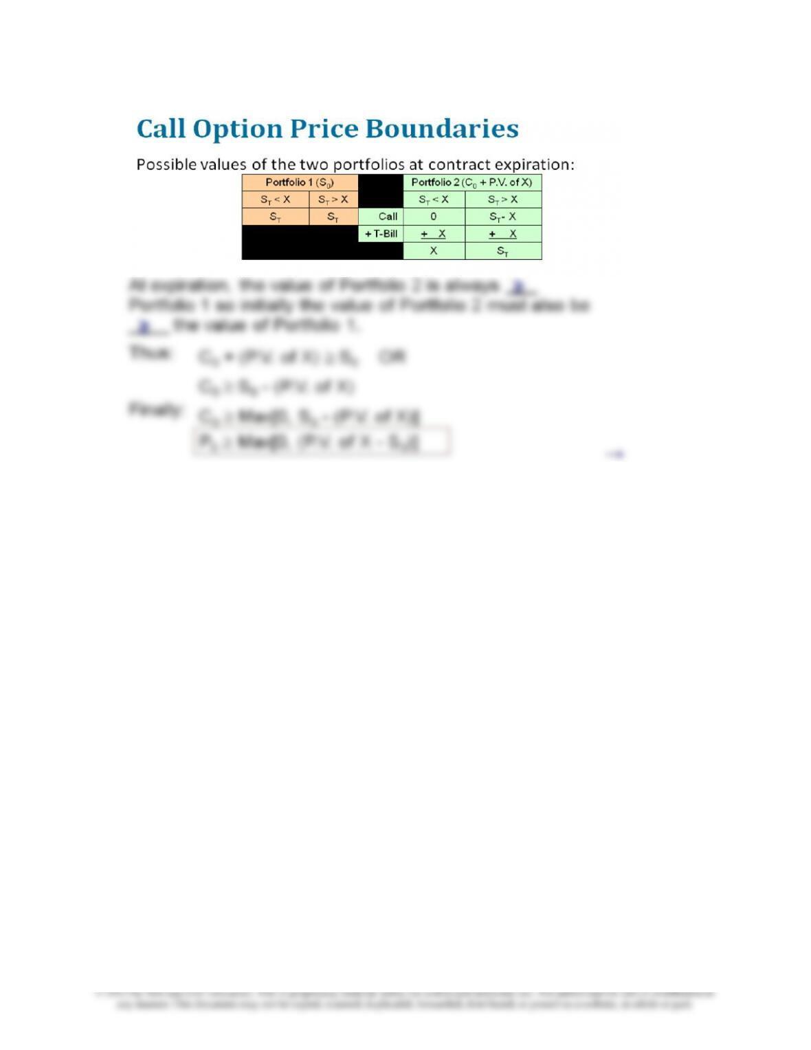
From here we can present the value of a call option at expiration and prior to expiration as
follows:
16–2
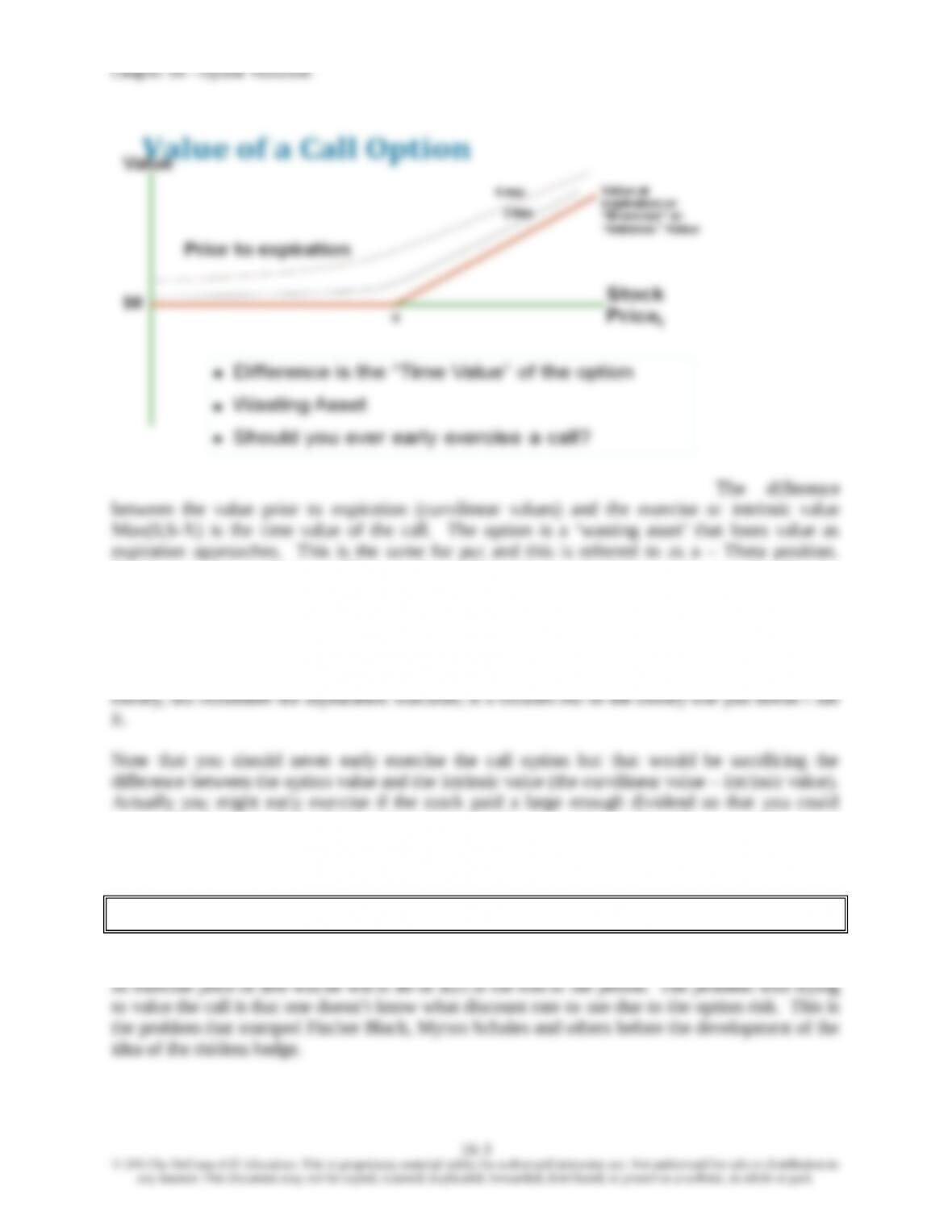
(Writing an option will be a + Theta position.) Going long or buying an option is a play that the
price will move enough before you run out of time value.
The time value of a call incorporates the probability that S will be in the money at period T given
S0, time to T, s2stock ,X, and the level of interest rates. The benefit of time value is the chance
that the option will wind up further in the money. Of course, it might not wind up further in the
receive the dividend. If the dividend is greater than the time value on the call, you would want to
early exercise right before the stock went ex-dividend.
2. Binomial Option Pricing
PPT 16-6 through PPT 16-12
A binomial pricing example is developed in the PPT. The example assumes the stock is currently
priced at $100 and will have a value of either $115or $85 at the end of the period. A call that has
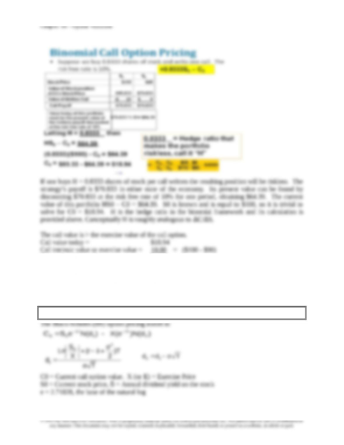
Time value of the call = $ 8.94
While the two-state approach is simplistic, the approach is easily generalized. Expansion of the
two-state approach shows how the probability distributions will approach the familiar bell shaped
curve as the number sub-periods increases.
3. Black-Scholes Option Valuation
PPT 16-13 through PPT 16-24
16–4
T = Time until expiration (not a point in time) in years,
σ = Annual standard deviation of continuously compounded stock returns
N(d) = probability that a random draw from a normal distribution will be less than d.
Including the annual dividend yield is an approximation of a discrete payment, (also technically the
dividend can’t be stochastic). It assumes no early exercise due to the dividend.
E(r) = (r + σ2/2)T when returns are lognormally distributed1
Ln (S0 / X) measures the continuous return needed for the stock to finish in the money
Roughly speaking the d1 numerator is a measure of the return needed to finish in the
money, the denominator measures this relative to the standard deviation of the returns.
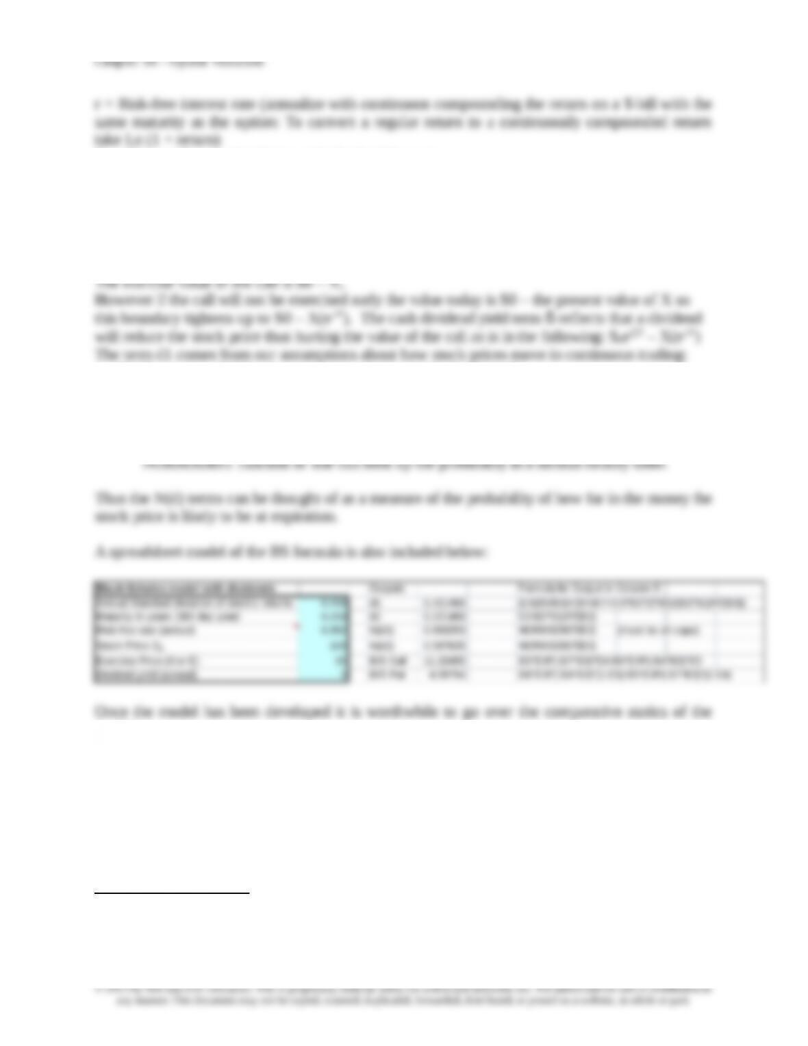
N(d) is cumulative normal probability. It can be calculated in Excel using the
model:
1The non continuously compounded returns are lognormally distributed. When we convert them to continuously compounded
returns rcont = Ln(1+rsimple), the rcont are normally distributed. If you have simple stock return series for monthly data or
shorter, you don’t need to do the conversion to continuous compounding because they will give you approximately the same
numbers (albeit this is a rule of thumb heuristic).
16–5
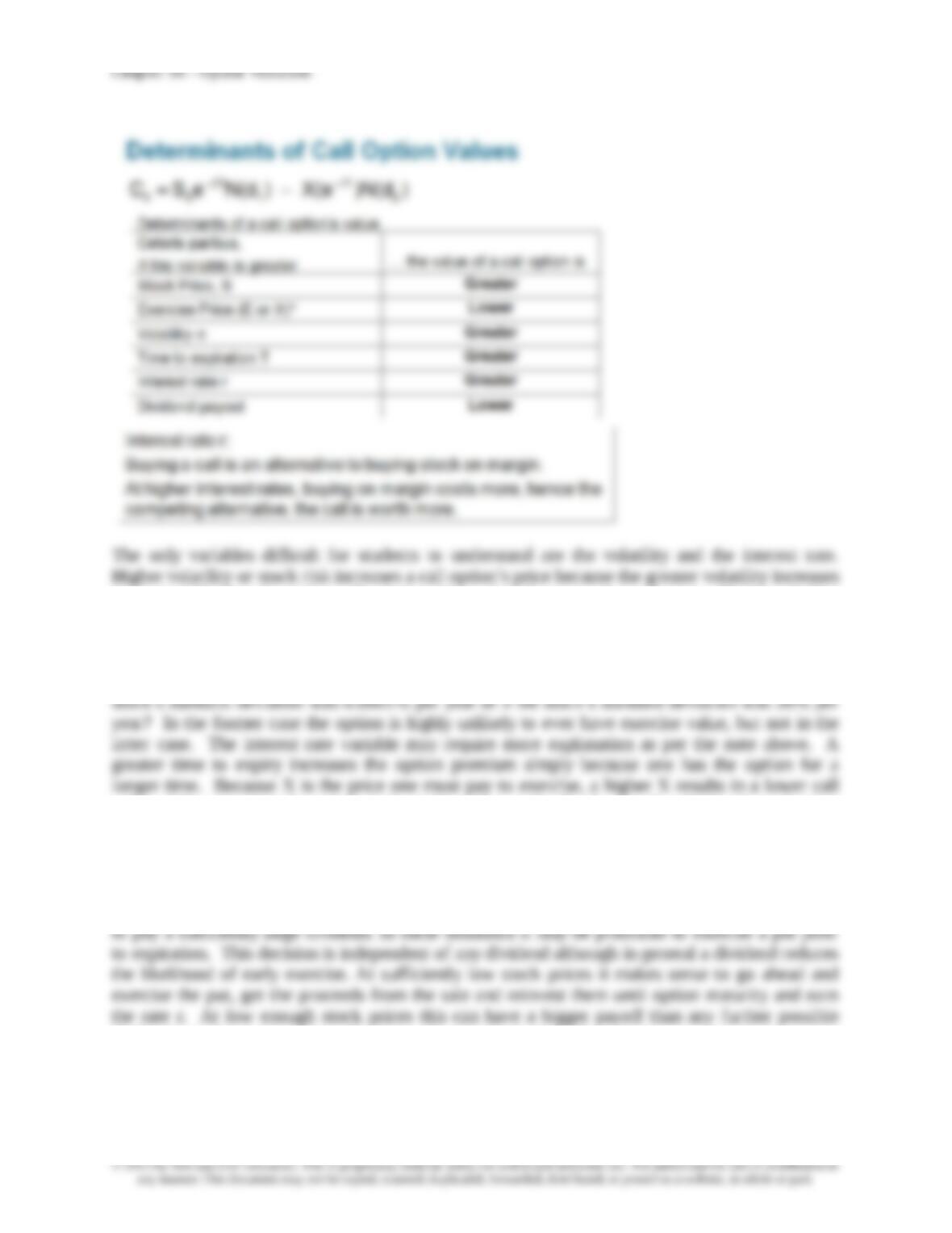
the probability that the option will wind up (deeper) in the money by expiration. Higher volatility
also indicates that the stock may not wind up in the money even if it currently is. However, due
to the asymmetric nature of options (one don’t use them if they don’t help) volatility increases
value. An extreme example might help here. Suppose one has a stock priced at $30 and a call
option on the stock with an exercise price of $50. Would one pay more for the option if the
value. Likewise since the option is the right to buy at the fixed value X, a higher S results in a
higher call value. Note that X would change if a stock split or stock dividend occurred, but not
otherwise. For instance, in a 2 for 1 stock split the exercise price would be halved. No adjustment
is made to X for a cash dividend.
As noted previously, a call option should not be exercised prior to maturity unless a stock is about
decline in stock price, and in such cases early exercise is desirable.
A version of the BS model is available for puts:
16–6
)]N(d [1eS )]N(d)[1X(e P 1
T
02
rT
0
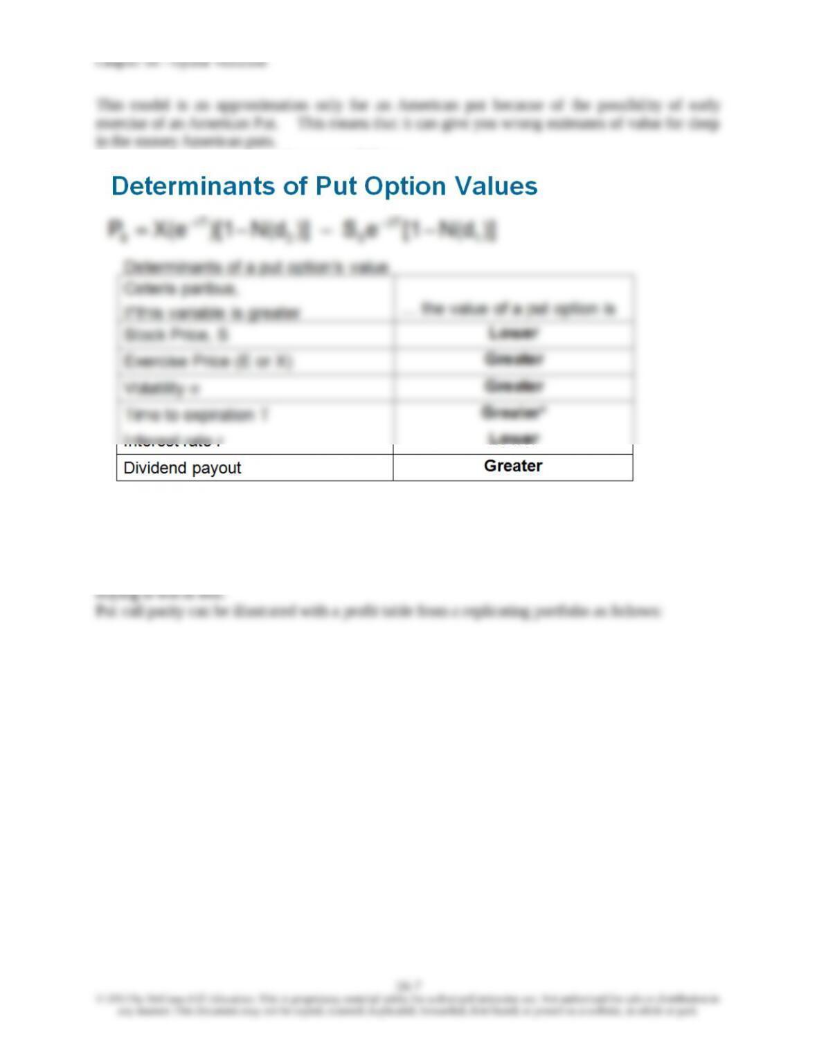
Determinants of put option values are as follows:
The interest rate variable probably requires some explanation. A higher interest rate lowers the PV
of X, thereby lowering the put value. In concept, the most you can get from a put is X, and the
lower the PV of X the lower the value of the put. Buying a put is conceptually equivalent to
shorting the stock and investing the proceeds in X. With a higher interest rate the bond one is
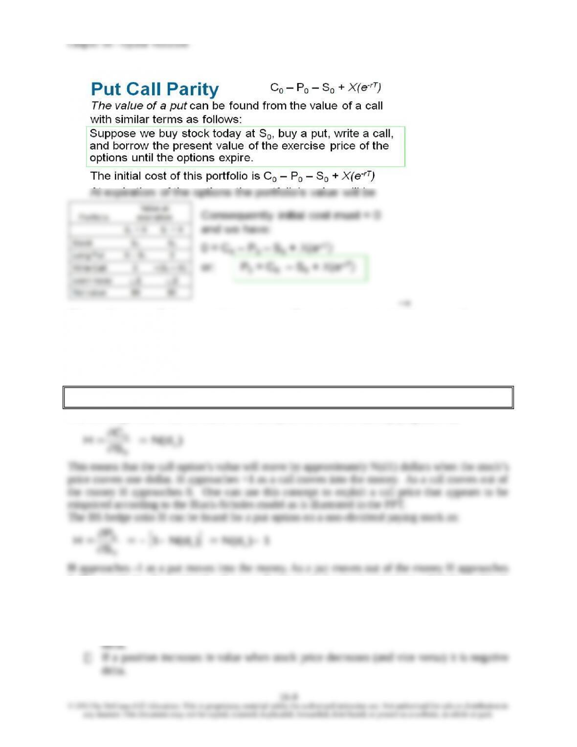
This combination will always result in a zero payoff at expiration so its initial cost must be zero as
well. This establishes the time zero value of 0 = C0-P0-S0 + X(e-rT). Knowing the call value and
the other variables one can find the implied put value. Using the BS model for puts will give the
same value. Both are correct only for European puts if there is a possibility of early exercise.
4. Using the Black-Scholes Formula
PPT 16-25 through PPT 16-32
The BS hedge ratio H can be found for a call option on a non-dividend paying stock as:
0. The sensitivity of a position’s value to a change in stock price is sometimes called the position’s
Delta.
If the position is not affected by a change in stock price the position has a delta of zero and is said
to be delta neutral.
If a position increases in value when stock price increases (and vice versa) it is positive
)d(N
S
C
H 1
0
0
Chapter 16 – Option Valuation
The position delta can be strategically manipulated as market conditions change and this idea is
the basis for portfolio insurance strategies accomplished through dynamic hedging. The basic
concept of portfolio insurance involves the purchase of protective puts. Purchase of protective
puts is a relatively easy concept but there are some limitations to the implementation of portfolio
option price per 1% change in stock price would not be atypical. Further out of the money
options have greater elasticity, deep out options may have elasticities of 25% or more. Deep in
the money options may have elasticities as low as 2-3% but they have to be deep in.
The stock’s standard deviation is the one variable in the BS model that is not easily observable.
The BS model can be used to find the implied volatility of the underlying stock, IF one is willing
5. Empirical Evidence
PPT 33
The B-S model has been heavily tested with the general conclusion that the model generates
option values that are very close to actual market prices. However, there are some problems with