Unlock document.
This document is partially blurred.
Unlock all pages and 1 million more documents.
Get Access
Chapter 13: Risk and Capital Budgeting
13-21
b. Recalculate the net present value of the Australian Mine at a
15 percent discount rate.
Years
Cash Flow
n Factor
PVIFA @ 15%
Present
Value
5–15
$300,000
(15 – 4)
(5.847 – 2.855)
$ 897,600
16–25
$500,000
(25 – 15)
(6.464 – 5.847)
$ 308,500
Present Value of inflows $1,206,100
Present Value of outflows $1,600,000
Net Present Value $ (393,900)
Now the decision should be made to reject the purchase of the
Australian Mine and purchase the U.S. Mine.
19. Coefficient of variation and investment decision (LO1) Mr. Sam Golff desires to invest
a portion of his assets in rental property. He has narrowed his choices down to two
apartment complexes, Palmer Heights and Crenshaw Village. After conferring with the
present owners, Mr. Golff has developed the following estimates of the cash flows for these
properties.
Palmer Heights
Crenshaw Village
Yearly Aftertax
Cash Inflow
(in thousands)
Probability
Yearly Aftertax
Cash Inflow
(in thousands)
Probability
$10 .................
.1
$15...............
.2
15 .................
.2
20...............
.3
30 .................
.4
30...............
.4
45 .................
.2
40...............
.1
50 .................
.1
a. Find the expected cash flow from each apartment complex.
b. What is the coefficient of variation for each apartment complex?
c. Which apartment complex has more risk?
13-19. Solution:
Chapter 13: Risk and Capital Budgeting
13-22
Mr. Sam Golff
D DP=
Palmer Heights
Crenshaw Village
D
P
DP
D
P
DP
10
.1
$1.0
15
.2
$ 3.0
15
.2
3.0
20
.3
6.0
30
.4
12.0
30
.4
12.0
45
.2
9.0
40
.1
4.0
50
.1
5.0
Expected Cash
Flow
$30.0
(thousands)
Expected Cash
Flow
$25.0
(thousands)
13-19. (Continued)
b. First find the standard deviation and then the coefficient of
variation.
V= D
Palmer Heights
D
D
(D D)−
2
(D D)−
P
2
(D D)−
P
$10
$30
$–20
$400
.10
40
15
30
–15
225
.20
45
30
30
0
0
.40
0
45
30
+15
225
.20
45
50
30
+20
400
.10
40
170
170 $13.04 (thousands)
==

Chapter 13: Risk and Capital Budgeting
13-23
V= $13.04/$30 = .435
Crenshaw Village
D
D
(D D)−
2
(D D)−
P
2
(D D)−
P
$15
$25
$–10
$100
.20
20.0
20
25
–5
25
.30
7.5
30
25
+5
25
.40
10.0
40
25
+15
225
.10
22.5
$60.0
60 $7.75 (thousands)
==
V=$7.75/$25=.310
20. Risk-adjusted discount rate (LO3) Referring to problem 19, Mr. Golff is likely to hold
the complex of his choice for 25 years, and will use this time period for decision-making
purposes. Either apartment complex can be acquired for $200,000. Mr. Golff uses a risk-
adjusted discount rate when considering investments. His scale is related to the coefficient
of variation.
Coefficient
of Variation
Discount
Rate
0 – 0.20 ..............................
5%
0.21 – 0.40 ..............................
9
(cost of capital)
0.41 – 0.60 ..............................
13
Over 0.90 ..............................
16
a. Compute the risk-adjusted net present values for Palmer Heights and Crenshaw
Village. You can get the coefficient of correlation and cash flow figures (in
thousands) from the previous problem.
b. Which investment should Mr. Golff accept if the two investments are mutually
exclusive? If the investments are not mutually exclusive and no capital rationing is
involved, how would your decision be affected?
13-20. Solution:
Chapter 13: Risk and Capital Budgeting
13-24
Mr. Sam Golff (Continued)
a. Risk-adjusted net present value
Palmer Heights
With V = .435,
discount rate = 13%
Crenshaw Village
With V = .310,
discount rate = 9%
Expected Cash Flow
$ 30,000
$ 25,000
IFPVA (n = 25)
7.330
9.823
Present Value of
Inflows
$219,900
$245,575
Present Value of
Outflows
200,000
$200,000
Net Present Value
$ 19,900
$ 45,575
13-20. (Continued)
b. If these two investments are mutually exclusive, he should
accept Crenshaw Village because it has a higher net present
value.
If the investments are non-mutually exclusive and no capital
rationing is involved, they both should be undertaken.
21. Decision-tree analysis (LO4) Allison’s Dresswear Manufacturers is preparing a strategy
for the fall season. One alternative is to expand its traditional ensemble of wool sweaters.
A second option would be to enter the cashmere sweater market with a new line of high-
quality designer label products. The marketing department has determined that the wool
and cashmere sweater lines offer the following probability of outcomes and related
cash flows.
Chapter 13: Risk and Capital Budgeting
13-25
Expand Wool
Sweaters Line
Enter Cashmere
Sweaters Line
Expected
Sales
Probability
Present Value
of Cash Flows
from Sales
Probability
Present
Value of
Cash Flows
from Sales
Fantastic ...................
.2
$180,000
.4
$300,000
Moderate ..................
.6
130,000
.2
230,000
Low ..........................
.2
85,000
.4
0
The initial cost to expand the wool sweater line is $110,000. To enter the cashmere sweater
line the initial cost in designs, inventory, and equipment is $125,000.
a. Diagram a complete decision tree of possible outcomes similar to Figure 13–8. Note
that you are dealing with thousands of dollars rather than millions. Take the analysis
all the way through the process of computing expected NPV (last column for each
investment).
b. Given the analysis in part a, would you automatically make the investment indicated?
Chapter 13: Risk and Capital Budgeting
13-26
13-21. Solution:
Allison’s Dresswear Manufacturers
a.
(1)
(2)
(3)
(4)
(5)
(6)
Expected
Sales
Probability
Present Value
of cash flows
from sales
Initial cost
NPV
(3) – (4)
Expected
NPV
(2) × (5)
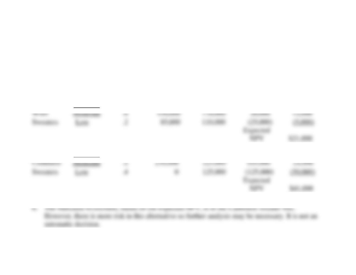
Expand
Fantastic
.2
$180,000
$110,000
$70,000
$14,000
Wool
Moderate
.6
130,000
110,000
20,000
12,000
Sweaters
Low
.2
85,000
110,000
(25,000)
(5,000)
Expected
NPV
$21,000
Enter
Fantastic
.4
$300,000
$125,000
$175,000
$70,000
Cashmere
Moderate
.2
230,000
125,000
105,000
21,000
Sweaters
Low
.4
0
125,000
(125,000)
(50,000)
Expected
NPV
$41,000
Chapter 13: Risk and Capital Budgeting
13-27
22. Probability analysis with a normal curve distribution (LO4) When returns from a
project can be assumed to be normally distributed, such as those shown in Figure 13–6 on
page ___ (represented by a symmetrical, bell-shaped curve), the areas under the curve can
be determined from statistical tables based on standard deviations. For example, 68.26
percent of the distribution will fall within one standard deviation of the expected value
(
D
± 1σ). Similarly 95.44 percent will fall within two standard deviations (
D
± 2σ), and so
on. An abbreviated table of areas under the normal curve is shown here.
Number of σ’s
from Expected Value
+ or –
+ and –
0.5 .....................
0.1915
0.3830
1.0 .....................
0.3413
0.6826
1.5 .....................
0.4332
0.8664
1.96 ...................
0.4750
0.9500
2.0 .....................
0.4772
0.9544
Assume Project A has an expected value of $30,000 and a standard deviation (σ) of $6,000.
a. What is the probability that the outcome will be between $24,000 and $36,000?
b. What is the probability that the outcome will be between $21,000 and $39,000?
c. What is the probability that the outcome will be at least $18,000?
d. What is the probability that the outcome will be less than $41,760?
e. What is the probability that the outcome will be less than $27,000 or greater than
$39,000?
13-22. Solution:
a. expected value = $30,000, σ = $6,000
Chapter 13: Risk and Capital Budgeting
13-28
13-22. (Continued)
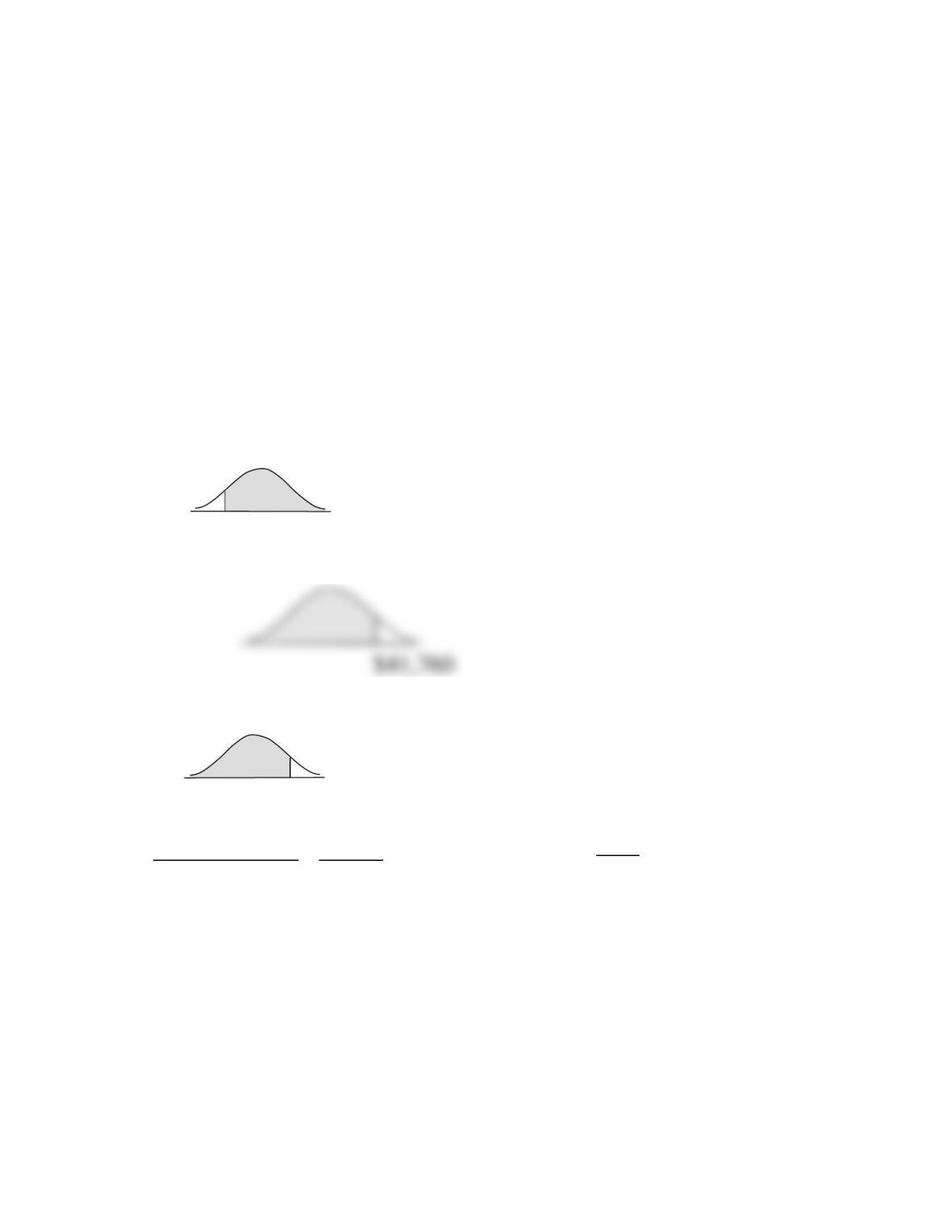
c. at least $18,000
$18,000 $30,000 $12,000 2
$6,000 $6,000
−−
= = −
d. Less than $41,760
$41,760 $30,000 $11,760 1.96
$6,000 $6,000
−==
$18,000
$41,760
.4772
.5000
.9772
Distribution
under the curve
.4750
.5000
.9750
Distribution
under the curve

Chapter 13: Risk and Capital Budgeting
13-29
13-22. (Continued)
e. Less than $27,000 or greater than $39,000
Area
$27,000 $30,000 $3,000 .5 .1915 .5000 .1915 = .3085
$6,000 $6,000
$39,000 $30,000 $9,000 .0668
1.5 .4332 .5000 .4332 =
$6,000 $6,000 .3753
−−
= = − −
−= = −
Distribution under the curve is .3753
23. Increasing risk over time (LO1) The Oklahoma Pipeline Company projects the following
pattern of inflows from an investment. The inflows are spread over time to reflect delayed
benefits. Each year is independent of the others.
Year 1
Year 5
Year 10
Cash
Inflow
Probability
Cash Inflow
Probability
Cash
Inflow
Probability
65 ..............
.20
50.......
.25
40 .........
.30
80 ..............
.60
80.......
.50
80 .........
.40
95 ..............
.20
110.......
.25
120 .........
.30
The expected value for all three years is $80.
a. Compute the standard deviation for each of the three years.
b. Diagram the expected values and standard deviations for each of the three years in a
manner similar to Figure 13–6.
c. Assuming 6 percent and 12 percent discount rates, complete the table below for
present value factors.
Year
PVIF
6%
PVIF
12%
Difference
1 ........
.943
.893
.050
5 ........
________
________
________
10 ........
________
________
________
$27,000
$39,000
Chapter 13: Risk and Capital Budgeting
13-30
d. Is the increasing risk over time, as diagrammed in part b, consistent with the larger
differences in PVIFs over time as computed in part c?
e. Assume the initial investment is $135. What is the net present value of the investment
at a 12 percent discount rate? Should the investment be accepted?
13-23. Solution:
Oklahoma Pipeline Company
a. Standard deviation—year 1
D
D
(D D)−
2
(D D)−
P
2
(D D)−
P
$65
80
–15
225
.20
45
80
80
0
0
.60
0
95
80
+15
225
.20
45
90
90 9.49
==
Standard deviation—year 5
D
D
(D D)−
2
(D D)−
P
2
(D D)−
P
50
80
–30
900
.25
225
80
80
0
0
.50
0
110
80
+30
900
.25
225
450
450 21.21
==


