Chapter 13: Risk and Capital Budgeting
Chapter 13
Risk and Capital Budgeting
Discussion Questions
13-1.
If corporate managers are risk-averse, does this mean they will not take risks?
Explain.
Risk-averse corporate managers are not unwilling to take risks, but will require
a higher return from risky investments. There must be a premium or additional
compensation for risk taking.
13-2.
Discuss the concept of risk and how it might be measured.
Risk may be defined in terms of the variability of outcomes from a given
investment. The greater the variability, the greater the risk. Risk may be
measured in terms of the coefficient of variation, in which we divide the
standard deviation (or measure of dispersion) by the mean. We also may
measure risk in terms of beta, in which we determine the volatility of returns on
an individual stock relative to a stock market index.
13-3.
When is the coefficient of variation a better measure of risk than the standard
deviation?
The standard deviation is an absolute measure of dispersion while the
coefficient of variation is a relative measure and allows us to relate the standard
deviation to the mean. The coefficient of variation is a better measure of
dispersion when we wish to consider the relative size of the standard deviation
or compare two or more investments of different size.
13-4.
Explain how the concept of risk can be incorporated into the capital budgeting
process.
Risk may be introduced into the capital budgeting process by requiring higher
returns for risky investments. One method of achieving this is to use higher
discount rates for riskier investments. This risk-adjusted discount rate approach
specifies different discount rates for different risk categories as measured by the
coefficient of variation or some other factor. Other methods, such as the
certainty equivalent approach, also may be used.
Chapter 13: Risk and Capital Budgeting
13-2
13-5.
If risk is to be analyzed in a qualitative way, place the following investment
decisions in order from the lowest risk to the highest risk:
a. New equipment.
b. New market.
c. Repair of old machinery.
d. New product in a foreign market.
e. New product in a related market.
f. Addition to a new product line.
Referring to Table 13-3, the following order would be correct:
repair old machinery (c)
new equipment (a)
addition to normal product line (f)
new product in related market (e)
completely new market (b)
new product in foreign market (d)
13-6.
Assume a company, correlated with the economy, is evaluating six projects, of
which two are positively correlated with the economy, two are negatively
correlated, and two are not correlated with it at all. Which two projects would
you select to minimize the company’s overall risk?
In order to minimize risk, the firm that is positively correlated with the
economy should select the two projects that are negatively correlated with the
economy.
13-7.
Assume a firm has several hundred possible investments and that it wants to
analyze the risk-return trade-off for portfolios of 20 projects. How should it
proceed with the evaluation?
The firm should attempt to construct a chart showing the risk-return
characteristics for every possible set of 20. By using a procedure similar to that
indicated in Figure 13-11, the best risk-return trade-offs or efficient frontier can
be determined. We then can decide where we wish to be along this line.
Chapter 13: Risk and Capital Budgeting
13-8.
Explain the effect of the risk-return trade-off on the market value of common
stock.
High profits alone will not necessarily lead to a high market value for common
stock. To the extent large or unnecessary risks are taken, a higher discount rate
and lower valuation may be assigned to our stock. Only by attempting to match
the appropriate levels for risk and return can we hope to maximize our overall
value in the market.
13-9.
What is the purpose of using simulation analysis?
Simulation is one way of dealing with the uncertainty involved in forecasting
the outcomes of capital budgeting projects or other types of decisions. A Monte
Carlo simulation model uses random variables for inputs. By programming the
computer to randomly select inputs from probability distributions, the outcomes
generated by a simulation are distributed about a mean and instead of
generating one return or net present value, a range of outcomes with standard
deviations are provided.
Chapter 13
Problems
1. Risk Averse (LO2) Assume you are risk averse and have the following three choices.
Which project will you select? Compute the coefficient of variation for each.
Expected
Value
Standard
Deviation
A
$1,800
$900
B
2,000
1,400
C
1,500
500
13–1. Solution:
VD
=

Chapter 13: Risk and Capital Budgeting
13-4
is the least risky.
2. Expected value and standard deviation (LO1) Lowe Technology Corp. is evaluating the
introduction of a new product. The possible levels of unit sales and the probabilities of their
occurrence are given:
Possible
Market Reaction
Sales
in Units
Probabilities
Low response ……………………………………
20
.10
Moderate response …………………………….
40
.20
High response …………………………………..
65
.40
Very high response…………………………….
80
.30
a. What is the expected value of unit sales for the new product?
b. What is the standard deviation of unit sales?
13–2. Solution:
Lowe Technology Corp
a.
D DP=
D P DP
b.
( )
2
D D P
=−

Chapter 13: Risk and Capital Budgeting
D
D
(D D)−
2
(D D)−
P
2
(D D)−
P
20
60
–40
1,600
.10
160
40
60
–20
400
.20
80
65
60
+5
25
.40
10
80
60
+20
400
.30
120
370

Chapter 13: Risk and Capital Budgeting
13-6
b.
2
(D D) P
=−
D
D
(D D)−
2
(D D)−
P
2
(D D)−
P
50
90
–40
1,600
.10
160
70
90
–20
400
.40
160
90
90
0
0
.20
0
140
90
+50
2,500
.30
750
1070
1070 32.71
==
4. Coefficient of variation (LO1) Shack Homebuilders, Limited, is evaluating a new
promotional campaign that could increase home sales. Possible outcomes and probabilities
of the outcomes are shown below. Compute the coefficient of variation.
Possible Outcomes
Additional
Sales in Units
Probabilities
Ineffective campaign ………………..………..
40
.20
Normal response ……………………..……
60
.50
Extremely effective ………………….……….
140
.30
13–4. Solution:
Shack Homebuilders, Limited
Coefficient of variation (V) = standard deviation/expected
value.
D DP=
D P DP
D

Chapter 13: Risk and Capital Budgeting
13-7
2
(D D) P
=−
D
D
(D D)−
2
(D D)−
P
2
(D D)−
P
40
80
–40
1,600
.20
320
60
80
–20
400
.50
200
140
80
+60
3,600
.30
1,080
1,600
1,600 40
==
40
V= .50
80 =
5. Coefficient of variation (LO1) Sam Sung is evaluating a new advertising program that
could increase electronics sales. Possible outcomes and probabilities of the outcomes are
shown below. Compute the coefficient of variation.
Possible Outcomes
Additional
Sales in Units
Probabilities
Ineffective campaign ………………………….
80
.20
Normal response …………………………..
124
.50
Extremely effective ………………..…………
340
.30
13–5. Solution:
Sam Sung
Coefficient of variation (V) = standard deviation/expected value.
D DP=
D P DP
80 .20 16

Chapter 13: Risk and Capital Budgeting
13-8
2
(D D) P
=−
D
D
(D D)−
2
(D D)−
P
2
(D D)−
P
80
180
–100
10,000
.20
2,000
124
180
–56
3,136
.50
1,568
340
180
+160
25,600
.30
7,680
11,248
11,248 106.06
==
106.06
V= .589
180 =
6. Coefficient of variation (LO1) Possible outcomes for three investment alternatives and
their probabilities of occurrence are given below.
Alternative 1
Outcomes Probability
Alternative 2
Outcomes Probability
Alternative 3
Outcomes Probability
Failure…………
50
.2
90
.3
80
.4
Acceptable …..
80
.4
160
.5
200
.5
Successful ……
120
.4
200
.2
400
.1
Rank the three alternatives in terms of risk from lowest to highest (compute the coefficient
of variation).
13–6. Solution:
Alternative 1
Alternative 2
Alternative 3
D × P = DP
D × P = P
D × P = DP
$50
0.2
$10
$90
0.3
$27
$80
0.4
$32
80
0.4
32
160
0.5
80
200
0.5
100
120
0.4
48
200
0.2
40
400
0.1
40
= $90
= $147
= $172
D
D

Chapter 13: Risk and Capital Budgeting
Standard Deviation Alternative 1
D
D
(D D)−
2
(D D)−
P
2
(D D)−
P
$ 50
$90
$–40
$1,600
.2
$320
80
90
–10
100
.4
40
120
90
+30
900
.4
360
$720
$ 90
$147
200
147
$ 80
$172
$ 8,464
$3,385.60
200
+28
784
392.00
400
51,984
$8,976.00
Chapter 13: Risk and Capital Budgeting
13-10
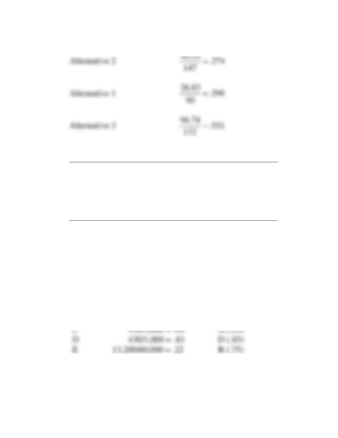
Alternative 2
40.26 .274
147 =
Alternative 1
26.83 .298
90 =
Alternative 3
94.74 .551
172 =
7. Coefficient of variation (LO1) Five investment alternatives have the following returns and
standard deviations of returns.
Alternatives
Returns:
Expected Value
Standard
Deviation
A ……………………………..
$ 1,200
$ 300
B ……………………………..
800
600
C ……………………………..
5,000
450
D ……………………………..
1,000
430
E ……………………………..
60,000
13,200
Using the coefficient of variation, rank the five alternatives from the lowest risk to the
highest risk.
13–7. Solution:
Coefficient of variation (V) = standard deviation/mean return
Ranking from lowest
to highest
A
300/1,200 = .25
C (.09)
B
600/800 = .75
E (.22)
C
450/5,000 = .09
A (.25)
D
430/1,000 = .43
D (.43)
E
13,200/60,000 = .22
B (.75)