Engineering Economy, 8th edition
Leland Blank and Anthony Tarquin
Chapter 19
More on Variation and Decision Making under Risk
Certainty, Risk, and Uncertainty
19.1 (a) Discrete
19.2 (a) Continuous (assumed) and uncertain
(b) Discrete with risk
19.3 Needed or assumed information to calculate an expected value:
Probability and Distributions
19.4 In $ million units,
19.5 Determine the probability values for C
C 0 1 2 3 4 ≥ 5
19.6 (a) Discrete as shown
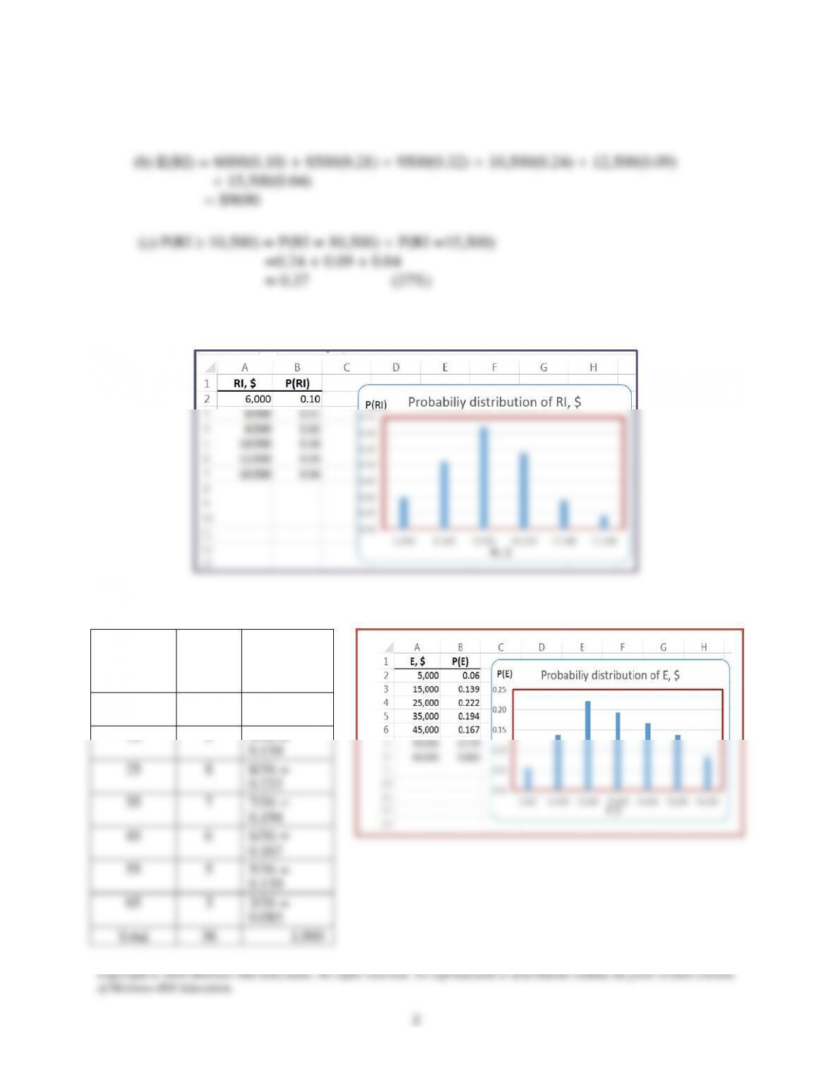
(d) Plot shown for observed values of Royalty Income, RI
19.7 (a) Calculate probabilities and plot the distribution. Using a spreadsheet, the result is:
45
6
6/36 =
Expense
range
midpoint,
E, $1000
Number
of
months
Probability,
P(E)
5
2
2/36 =
0.056
15
5
5/36 =
0.139
25
8
8/36 =
0.222
35
7
7/36 =
0.194
0.167
55
5
5/36 =
0.139
65
3
3/36 =
0.083
Total
36
1.000
(b) Can use months or probabilities; using probabilities
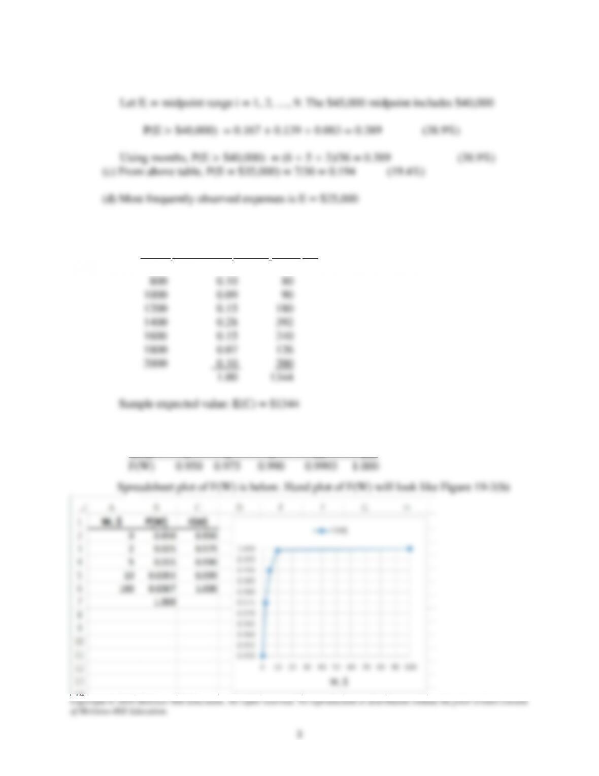
19.8 Use Equation [18.2] or [19.8] to find E(C)
Cell Ci, $ P(Ci) Ci × P(Ci), $
600 0.06 36
19.9 (a) W is discrete; plot W vs. F(W)
W, $ 0 2 5 10 100
(b) E(W) = 0.95(0) + … + 0.0007(100)
(c) 2.000 – 0.288 = $1.712
19.10 (a) P(N) = (0.5)N N = 1, 2, 3, …
N 1 2 3 4 5 etc.
5-2
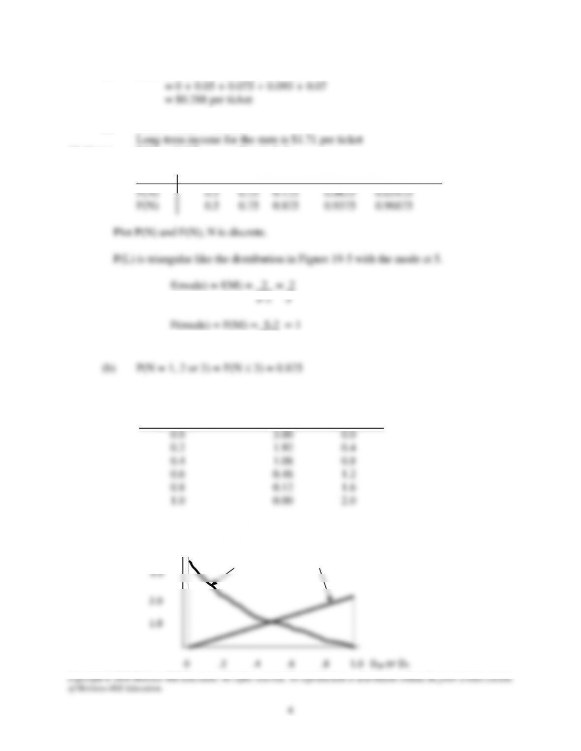
19.11 (a) Determine several values of DM and DY and plot.
DM or DY f(DM) f(DY)
f(DM) is a decreasing power curve and f(DY) is increasing linear.
f(D)
f(DM
)
f(DY
)
0 .2 .4 .6 .8 1.0 D
M
or D
Y
3.0
19.12 (a) Xi 1 2 3 6 9 10
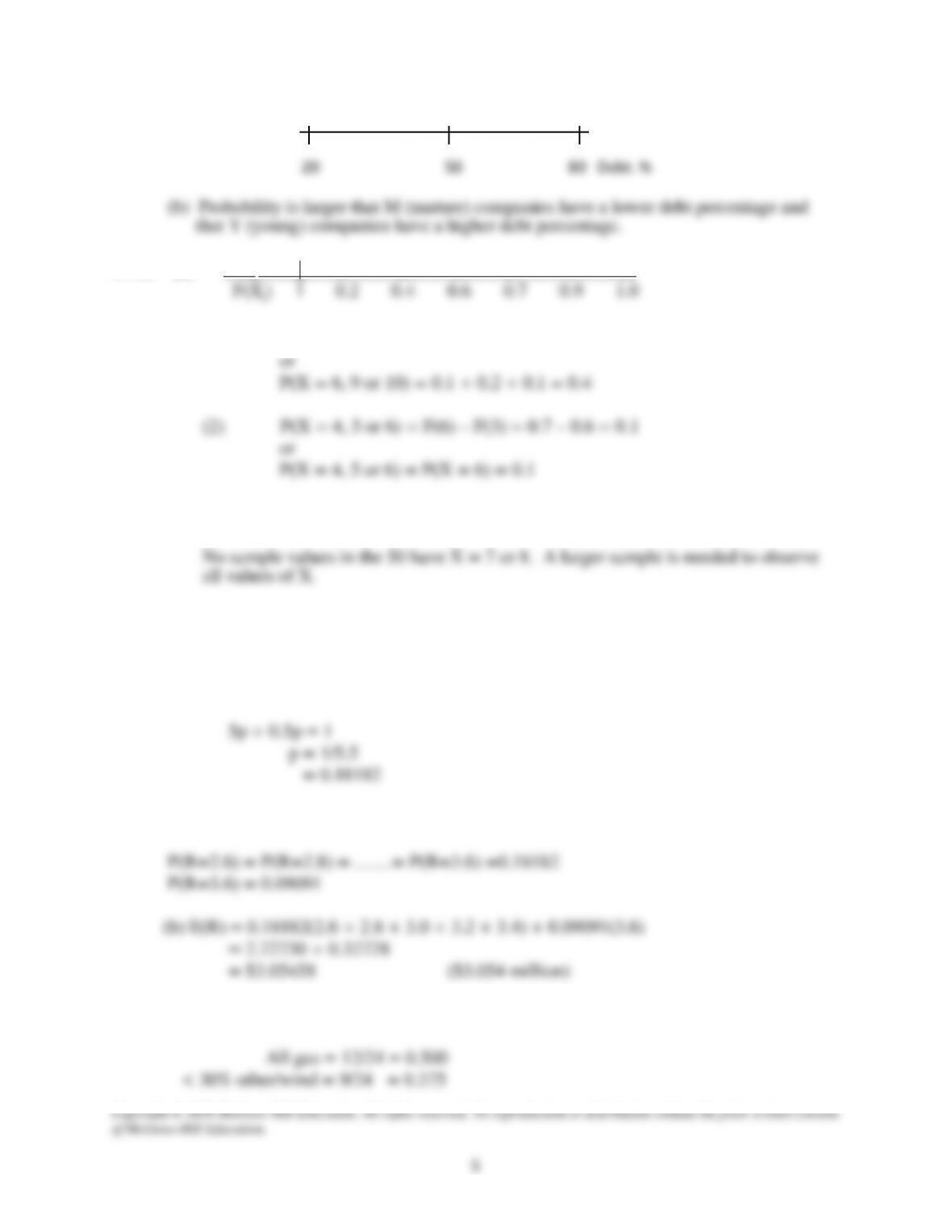
(b) (1) P(6 ≤ X ≤ 10) = F(10) – F(3) = 1.0 – 0.6 = 0.4
(c) P(X = 7 or 8) = F(8) – F(6) = 0.7 – 0.7 = 0.0
Random Samples
19.13 (a) Let p = probability such the 5p plus 1/2p equals 1.0
In $ million units for R, the probability statements are:
19.14 The probability of occurrence of each situation is as follows:
Copyright © 2018 McGraw–Hill Education. All rights reserved. No reproduction or distribution without the prior written consent
of McGraw–Hill Education.
6
≥ 30% other/wind = 3/24 = 0.125
E(R) = 5,270,000(0.50) + 7,850,000(0.375) + 12,130,000(0.125)
= $7,095,000
Difference = revenue – costs
= 7,095,000 – 6,800,000
= $295,000 greater than expenses
19.15 (a) Sample size is n = 40
(b) P(T=2) = 0.325 Stated P(T = 2) = 0.30 (close)
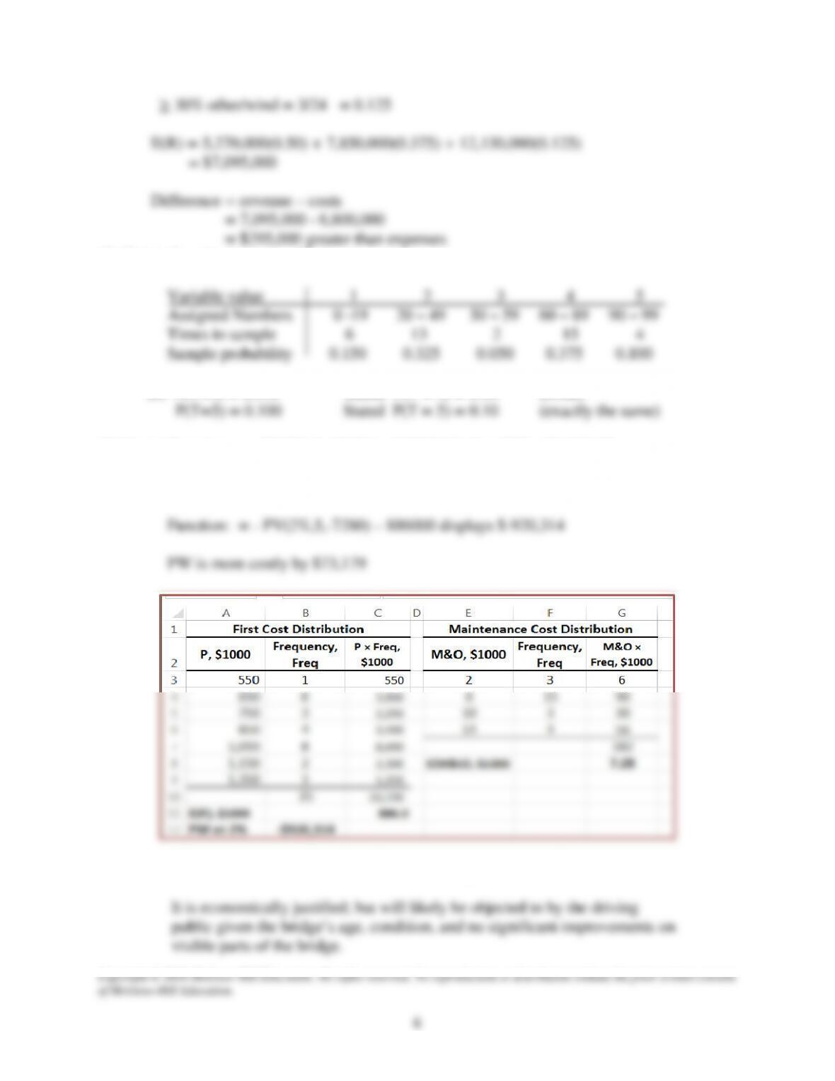
19.16 (a) Function: = – PV(2%,5,-10000) – 800000 displays PW = $-847,135
(b) Expected value computations: E(P) = $886,000 and E(M&O) = $7,280 per year
(c) Function: = – PV(2%,5,180000) – 800000 displays $48,423.
19.17 (a) X 0 0.2 0.4 0.6 0.8 1.0
19.18 (a) When the RAND( ) function was used for 100 values in column A of a spreadsheet,
Sample Estimates – Average and Standard Deviation
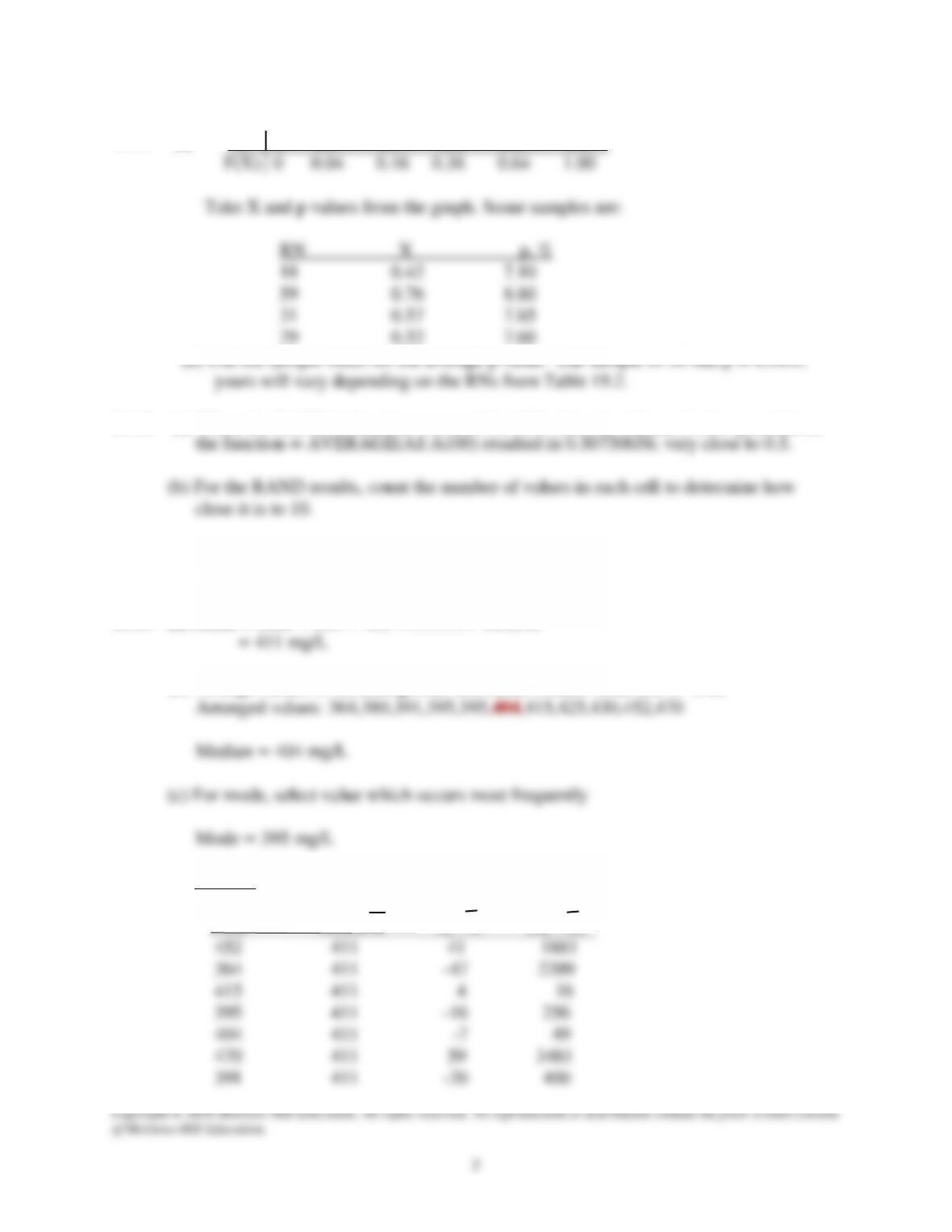
19.19 (a) Mean = (452 + 364 + 415 +………+ 380)/11
(b) Arrange values in increasing order and select middle value (i.e. 6th one)
(d) By hand:
COD Mean, X Xi – X (Xi – X)2
Copyright © 2018 McGraw–Hill Education. All rights reserved. No reproduction or distribution without the prior written consent
of McGraw–Hill Education.
8
395 411 -16 256
425 411 14 196
430 411 19 361
380 411 -31 961
4521 0 9866
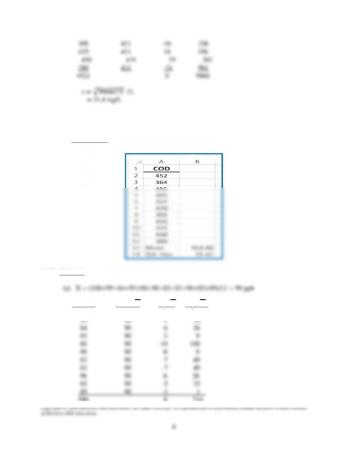
s = √9866/(11 -1)
= 31.4 mg/L
Spreadsheet:
19.20 By hand:
(b) Reading Mean, X Xi – X (Xi – X)2
108 90 18 324
990 0 710
Copyright © 2018 McGraw–Hill Education. All rights reserved. No reproduction or distribution without the prior written consent
of McGraw–Hill Education.
9
s = √710/(11 -1) = 8.43 ppb
(c) Range for ±1s is 90 ± 8.43 = 81.57– 98.43
Spreadsheet: Values entered into cells A1:A11
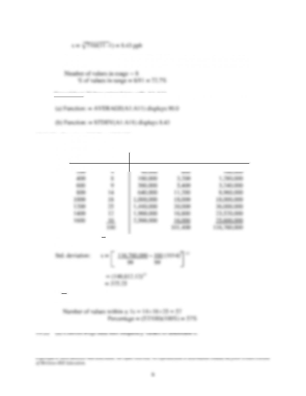
19.21 Use Equations [19.9] and [19.12].
Cell,
Xi fi Xi
2 fiXi fiXi
2
Sample mean: X = 101,400/100 = 1014.00
(b) X ± 1s is 1014.00 ± 375.25 = 638.75 and 1,389.25
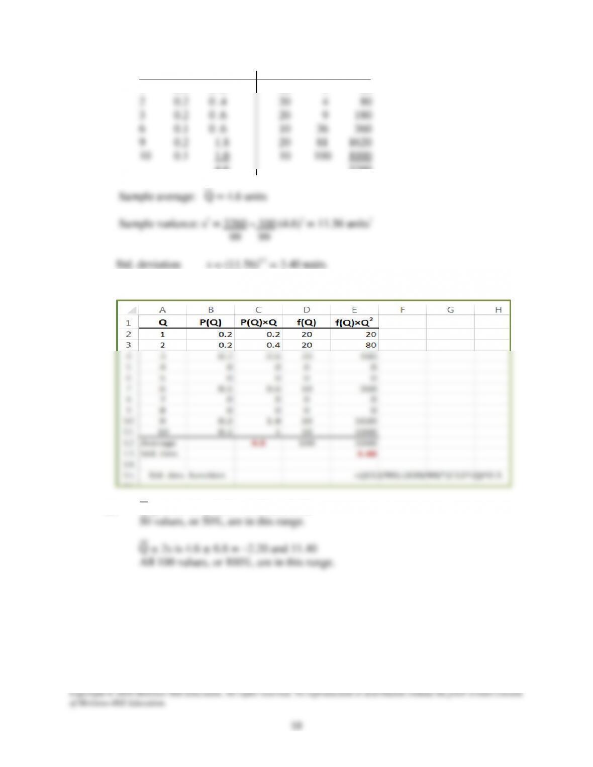
Q P(Q) QP(Q) f Q2 fQ2
1 0.2 0 .2 20 1 20
4.6 3260
(b) Average and standard deviation values are shown.
(c) Q ± 1s is 4.6 ± 3.40 = 1.20 and 8.00
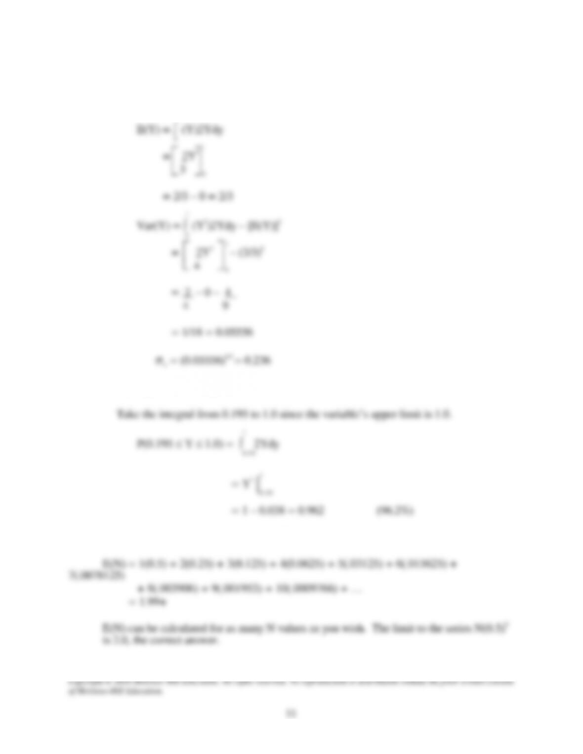
19.23 (a) Use Equations [19.15] and [19.16]. Substitute Y for DY.
f(Y) = 2Y
1
(b) E(Y) ± 2σ is 0.667 ± 0.472 = 0.195 and 1.139
19.24 Use Equation [19.8] where P(N) = (0.5)N
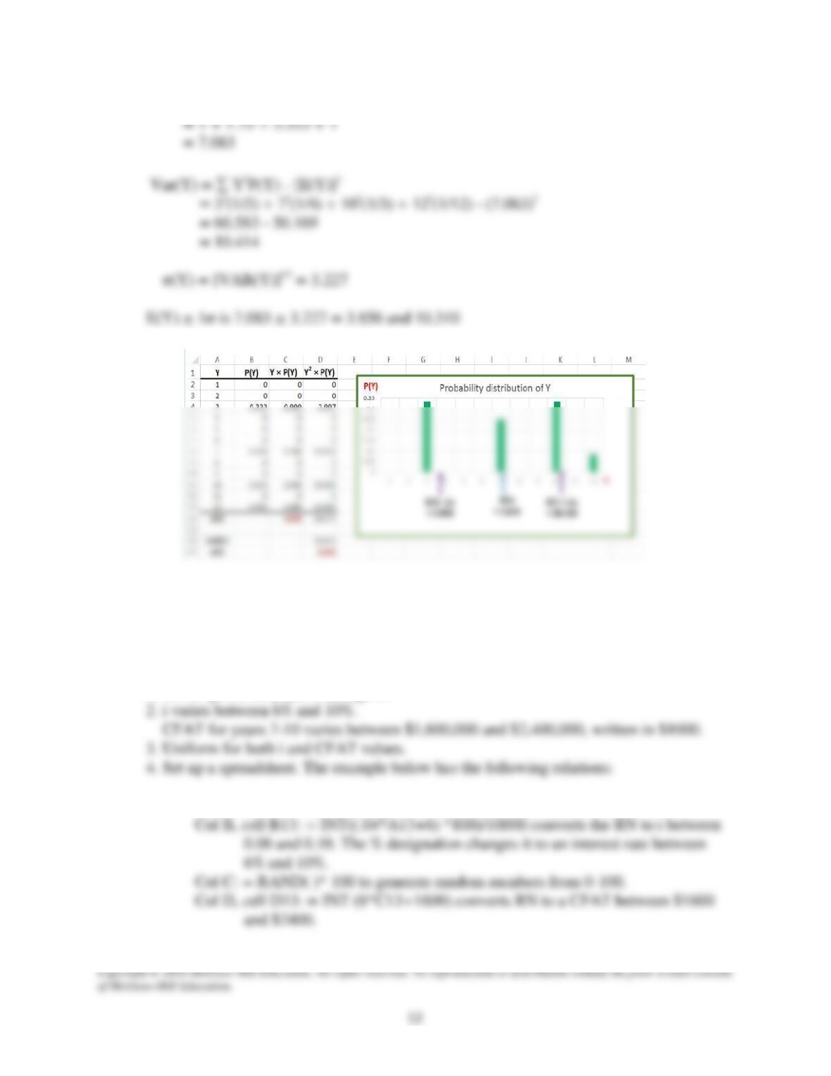
19.25 E(Y) = 3(1/3) + 7(1/4) + 10(1/3) + 12(1/12)
Simulation
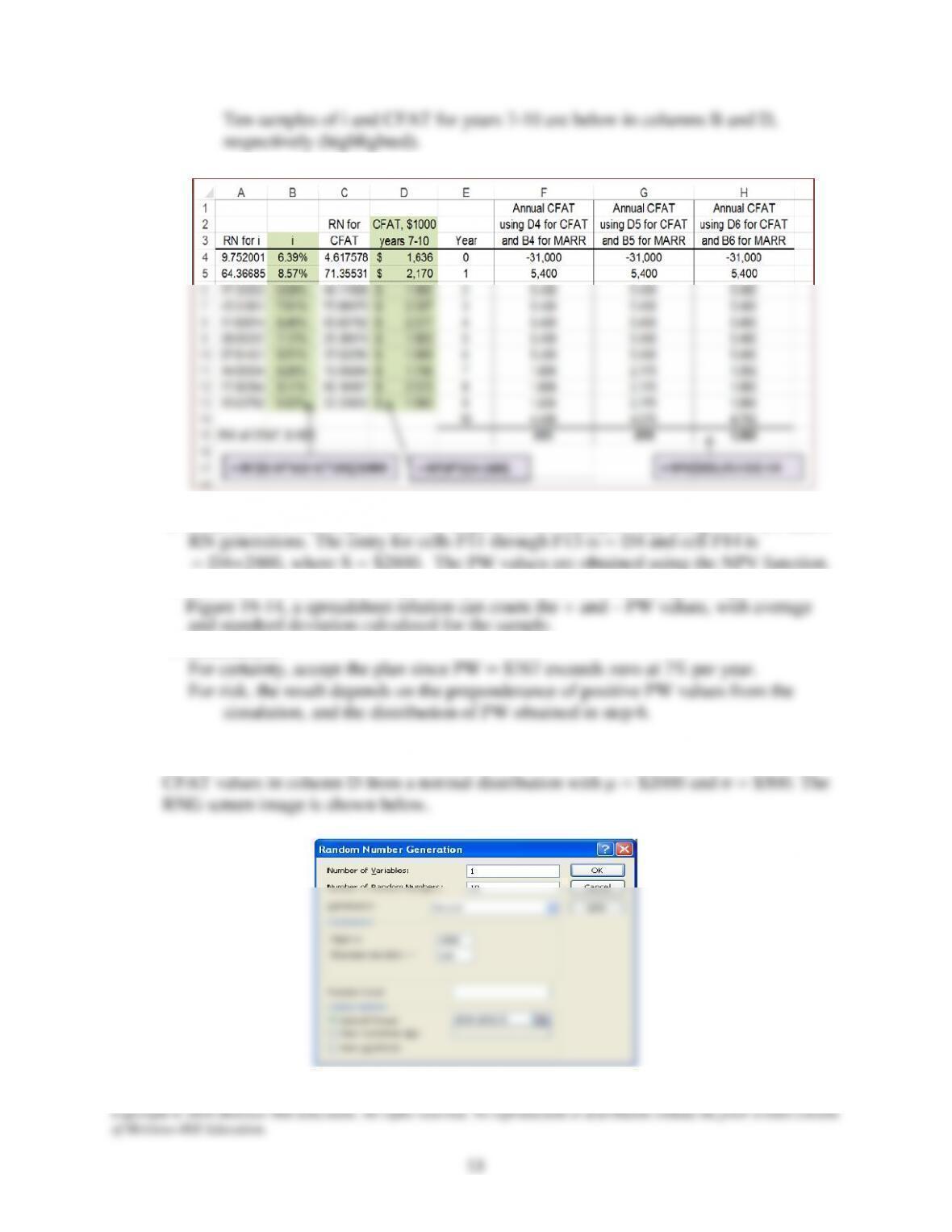
19.26 Using a spreadsheet, the steps in Sec. 19.5 are applied.
1. CFAT given for years 0 through 6.
Col A: = RAND ( )* 100 to generate random numbers from 0-100.
Copyright © 2018 McGraw–Hill Education. All rights reserved. No reproduction or distribution without the prior written consent
of McGraw–Hill Education.
13
Ten samples of i and CFAT for years 7-10 are below in columns B and D,
respectively (highlighted).
5. Columns F, G and H give 3 CFAT sequences, for example only, using rows 4, 5 and 6
6. Plot the PW values for as large a sample as desired. Or, following the logic of
7. Conclusion:
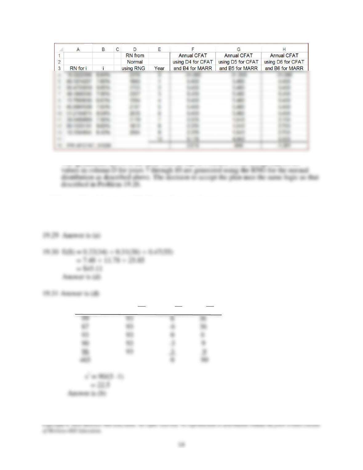
19.27 Use the spreadsheet Random Number Generator (RNG) on the tools toolbar to generate
Copyright © 2018 McGraw–Hill Education. All rights reserved. No reproduction or distribution without the prior written consent
of McGraw–Hill Education.
14
The spreadsheet above is the same form as that in Problem 19.26, except that CFAT
Additional Problems and FE Exam Review Questions
19.28 Answer is (c)
19.32 Reading Mean, X Xi – X (Xi – X)2
19.33 P(Income > $8500) = 0.32 + 0.24 + 0.09 + 0.04
19.34 s = √4,680,000/(12 -1)
19.35 Four numbers (52, 67, 74, and 50) are in the range 50 through 74, which indicate type C.
Solution to Case Study, Chapter 19
USING SIMULATION AND THREE-ESTIMATE SENSITIVITY ANALYSIS
This simulation is left to the learner. The 7–step procedure from Section 19.5 can be applied here.
Set up the RNG for the cash flow values of AOC, S, and n for each alternative. For each sample
cash flow series, calculate the AW value for each alternative. To obtain a final answer of which
alternative is the best, it is recommended that the number of positive and negative AW values be
counted as they are generated. Then the alternative with the most positive AW values indicates
which one to accept. Of course, due to the RNG generation of AOC, S and n values, this decision
may vary from one simulation run to the next.