Engineering Economy, 8th edition
Leland Blank and Anthony Tarquin
Chapter 18
Sensitivity Analysis and Staged Decisions
Sensitivity to Parameter Variation
$325,000: AW = -850,000(A/P,20%,5) + 325,000
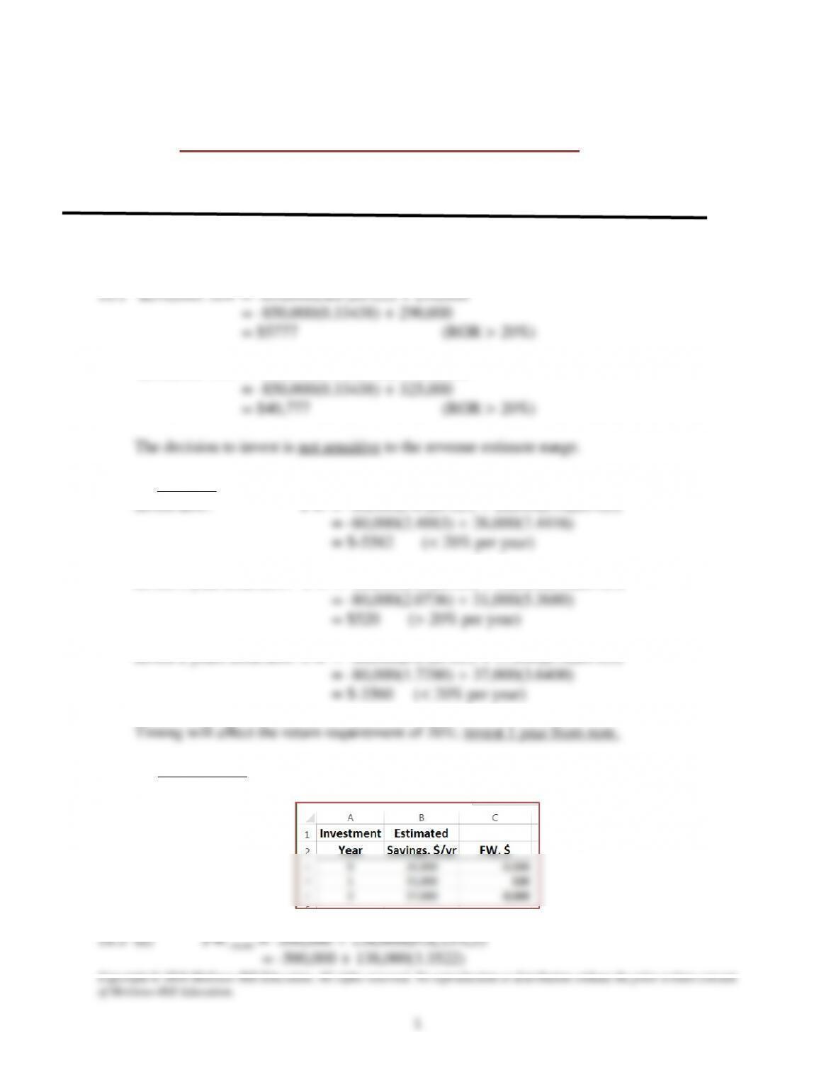
18.2 (a) By hand:
Invest now: FW = -80,000(F/P,20%,5) + 26,000(F/A,20%,5)
Invest 1 year from now: FW = -80,000(F/P,20%,4) + 31,000(F/A,20%,4)
Invest 2 years from now: FW = -80,000(F/P,20%,3) + 37,000(F/A,20%,3)
(b) Spreadsheet: Same result using the FV function = – FV(20%,n,savings,-80000)
Copyright © 2018 McGraw–Hill Education. All rights reserved. No reproduction or distribution without the prior written consent
of McGraw–Hill Education.
2
= $-37,396 (ROR < 15%)
PW165,000 = -500,000 + 165,000(P/A,15%,5)
= –500,000 + 165,000(3.3522)
= $53,113 (ROR > 15%)
The decision to invest is sensitive to the revenue estimates
(b) Function = PMT(15%,5,-500000) displays $149,158 per year
18.4 (a) AWcurrent = $–62,000
The decision is sensitive
(b) Replace when AW < $-62,000 for an S between $10,000 and $14,500. Set up the
18.5 PWlow = -80,000 + 10,000(P/F,8%,6) + 10,000(P/A,8%,6)
The $10,000 revenue estimate is the only one that does not favor the purchase. The
18.6 (a) PWLease = – 30(1000) – 30(1000)(P/A,20%,2)
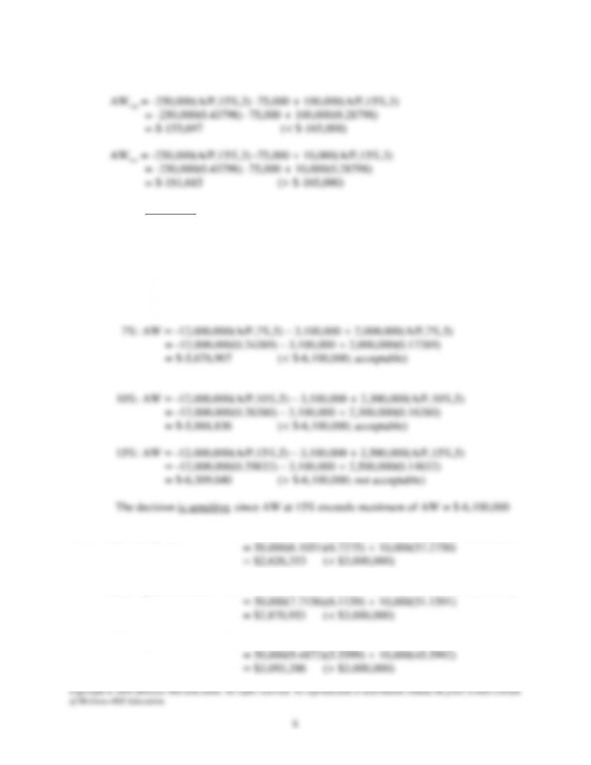
PWBuild,70 = -80,000 – 70(1000) + 120,000(P/F,20%,3)
PWBuild, 63 = -80,000 – 63(1000) + 120,000(P/F,20%,3)
The lease option is less expensive if the building cost is $70; lease is more
expensive for the $63 per m2 build option.
(b) Functions: Lease: = – PV(20%,2,-30000) -30000 displays $-75,833
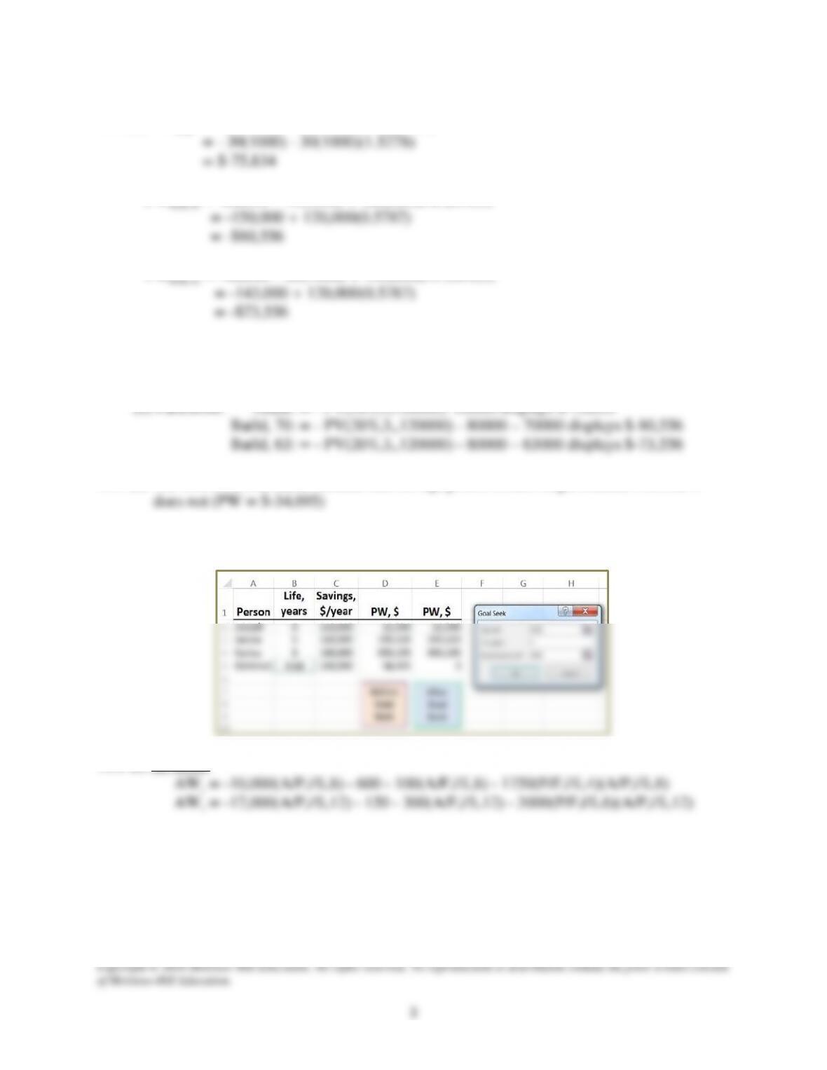
18.7 (a) The first three estimates indicate that the equipment should be purchased; Mehmet’s
(b) Use Goal Seek to change the life (cell B5) from 6 to 6.64 years so that PW = 0 (cell E5)
18.8 (a) By hand:
Calculate AW at each MARR value. The decision is sensitive to MARR, changing at
MARR = 6%.
(b) Spreadsheet: The PMT functions are shown; AW values are the same as by hand.
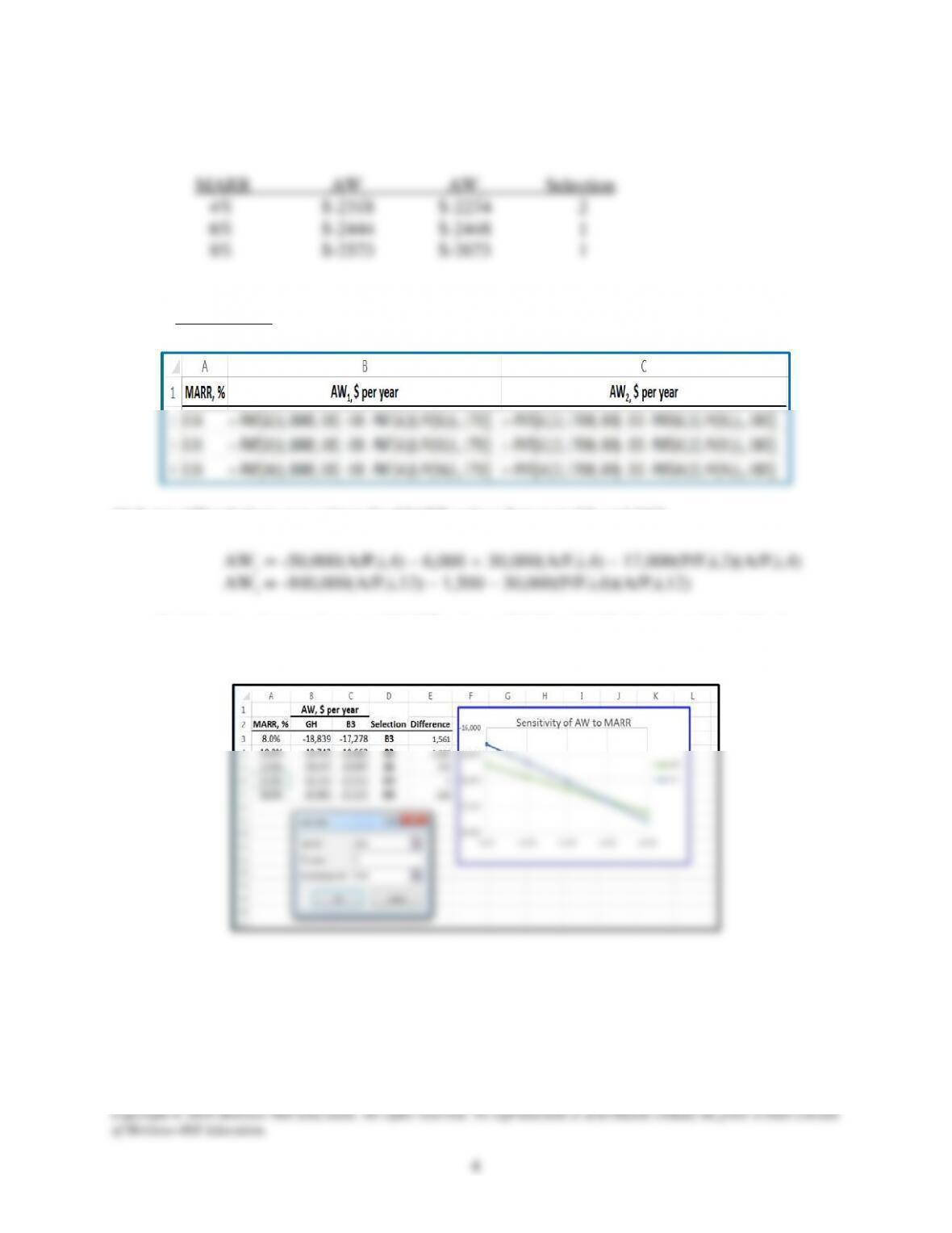
18.9 (a) AW relations are written for MARR values between 8% and 16%
(b) Selection changes between MARR values of 14% and 16%. Graph and Goal Seek
determine the MARR breakeven point at 13.9% per year.
18.10 AWcontract = $-165,000
Decision is sensitive to salvage value.
Total should estimate the salvage more closely before choosing between purchase and
subcontractor.
18.11 Required AW < $-6.1 million
18.12 Start family now: FW = 50,000(F/A,10%,5)(F/P,10%,20) + 10,000(F/A,10%,20)
Child 1 year from now: FW = 50,000(F/A,10%,6)(F/P,10%,19) + 10,000(F/A,10%,19)
Child 2 years from now: FW = 50,000(F/A,10%,7)(F/P,10%,18) + 10,000(F/A,10%,18)
18.13 (a) By hand:
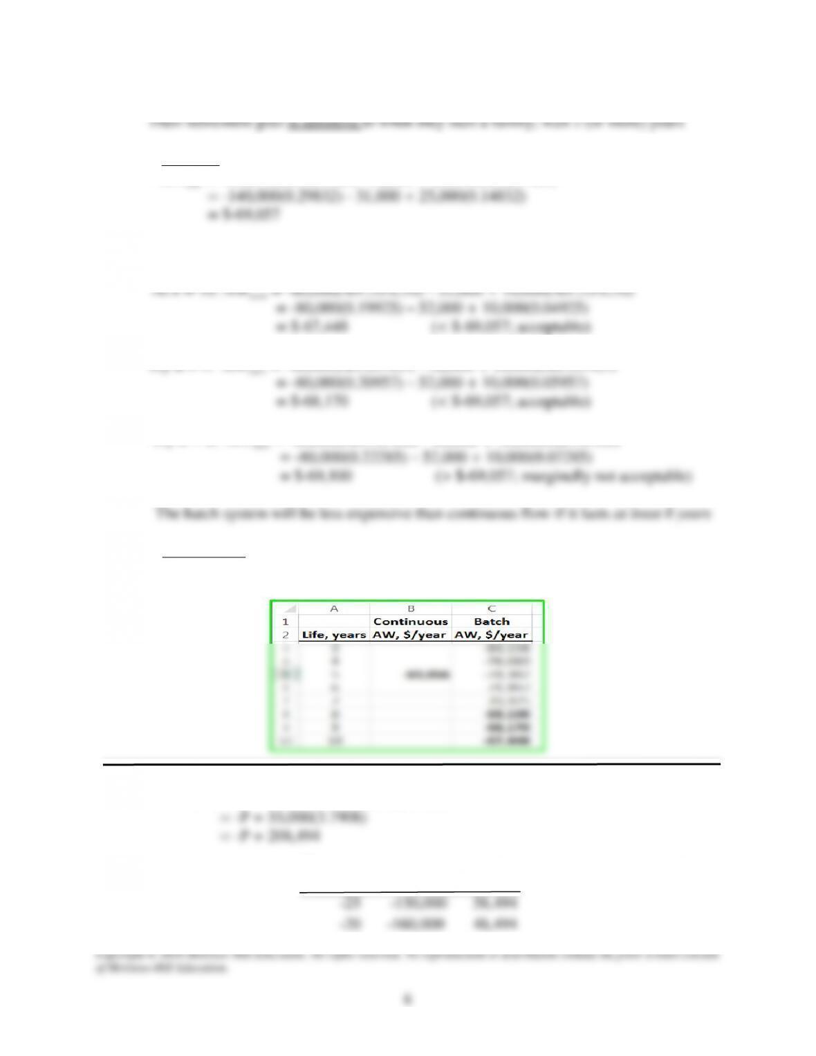
AWcont = -140,000(A/P,15%,5) – 31,000 + 25,000(A/F,15%,5)
The lowest cost for batch will occur when its life is longest, 10 years
Try n = 9: AWbatch = -80,000(A/P,15%,9) – 52,000 + 10,000(A/F,15%,9)
Try n = 8: AWbatch = –80,000(A/P,15%,8) – 52,000 + 10,000(A/F,15%,8)
(b) Spreadsheet: An expected life of slightly over 8 years is required to select the batch
process.
18.14 P = first cost
PW = –P + (60,000 – 5000)(P/A,10%,5)
Percent
variation
P value, $
PW, $
-25
-150,000
58,494
-20
-160,000
48,494
7
Sensitive at +10% increase in first cost when PW goes negative
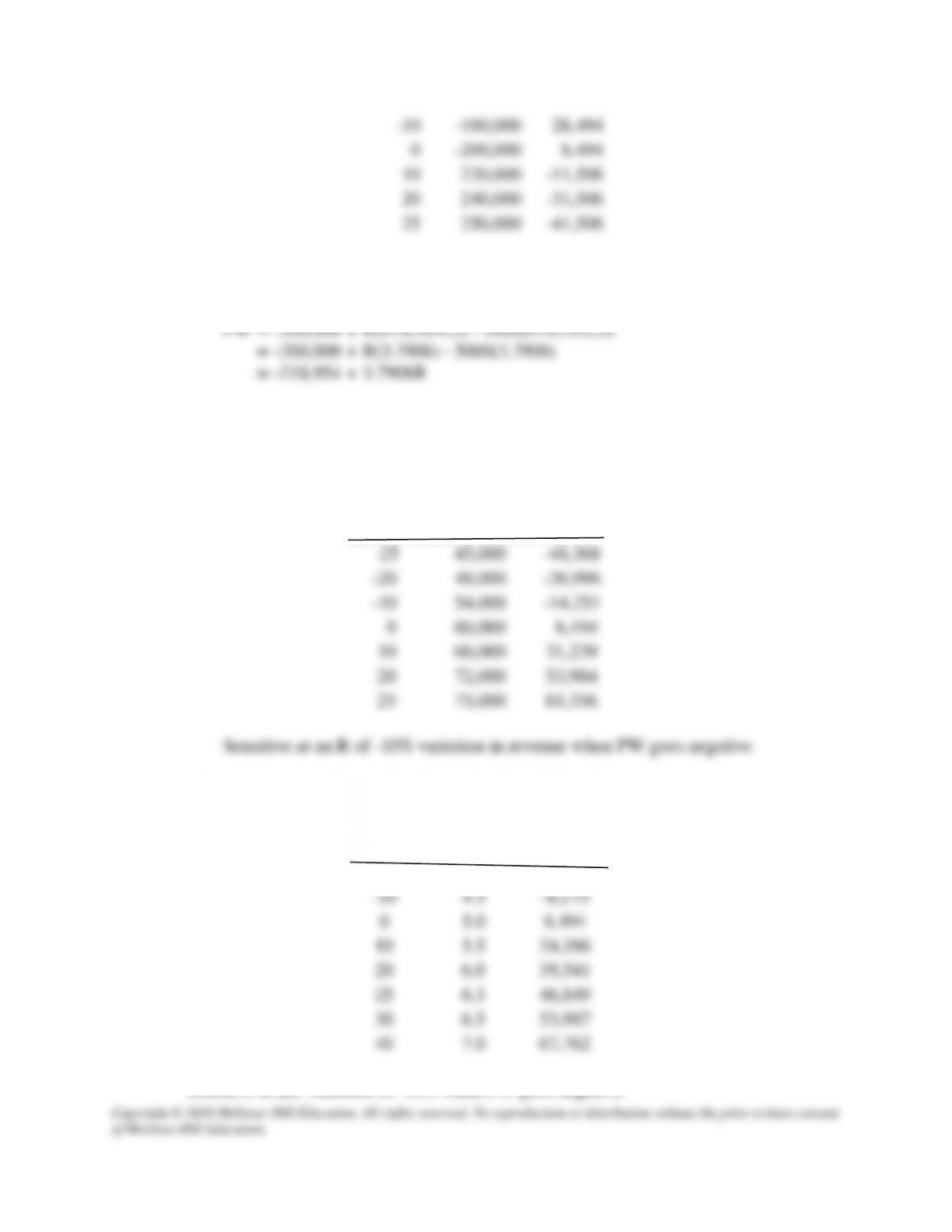
18.15 R = revenue
Percent
variation
R value, $
PW, $
-25
45,000
–48,368
-20
48,000
-36,996
-10
54,000
-14,251
0
60,000
8,494
10
66,000
31,239
20
72,000
53,984
25
75,000
65,356
18.16 n = life PW = –200,000 + (60,000 – 5000)((P/A,10%,n)
Percent
variation
n, years
PW, $
-20
4.0
–25,656
-10
4.5
-8,175
0
5.0
8,494
10
5.5
24,386
20
6.0
39,541
25
6.3
46,849
30
6.5
53,987
40
7.0
67,762
Sensitive at life variation of -10% when PW goes negative.
0
-200,000
8,494
10
220,000
-11,506
20
240,000
-31,506
25
250,000
-41,506
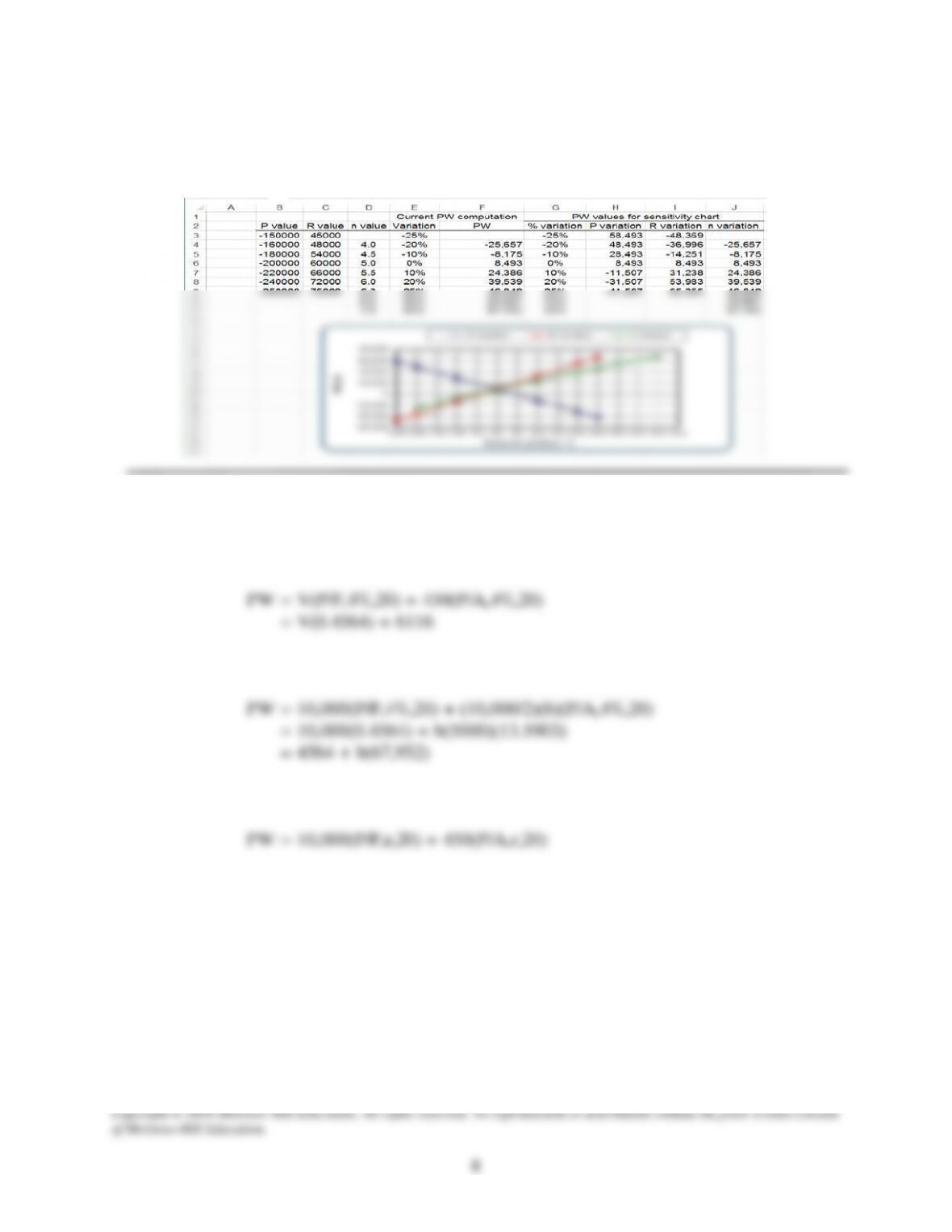
18.17 Spreadsheet and plot is for all three parameters: P, R and n. Variations in P and R have
about the same effect on PW in opposite directions, and slightly more effect than variation
in n.
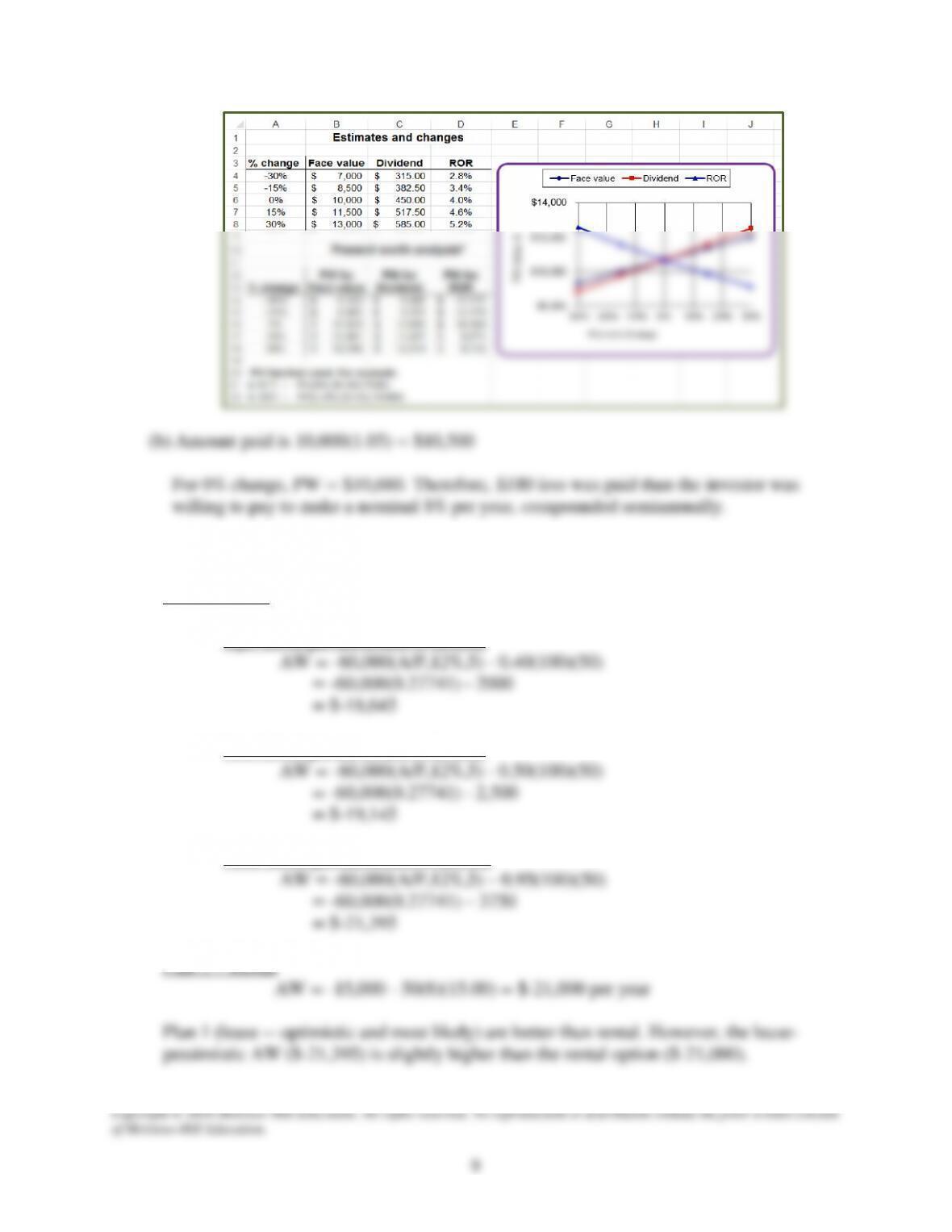
18.18 (a) PW calculates the amount you should be willing to pay now. Plot PW versus ±30%
changes in (1), (2) and (3) on one graph.
(1) V = face value; r is 4% per 6–month period
(2) b = dividend rate; r is 4% per 6–month period
(3) r = nominal rate per 6–month period
Copyright © 2018 McGraw–Hill Education. All rights reserved. No reproduction or distribution without the prior written consent
of McGraw–Hill Education.
9
(b) Amount paid is 10,000(1.05) = $10,500
For 0% change, PW = $10,680. Therefore, $180 less was paid than the investor was
willing to pay to make a nominal 8% per year, compounded semiannually.
Three–Estimate Sensitivity Analysis
18.19 Plan 1 – Lease
Opt: $0.40 per ton (AOC = $2000)
ML: $0.50 per ton (AOC = $2500)
Pess: $0.95 per ton (AOC = $3750)
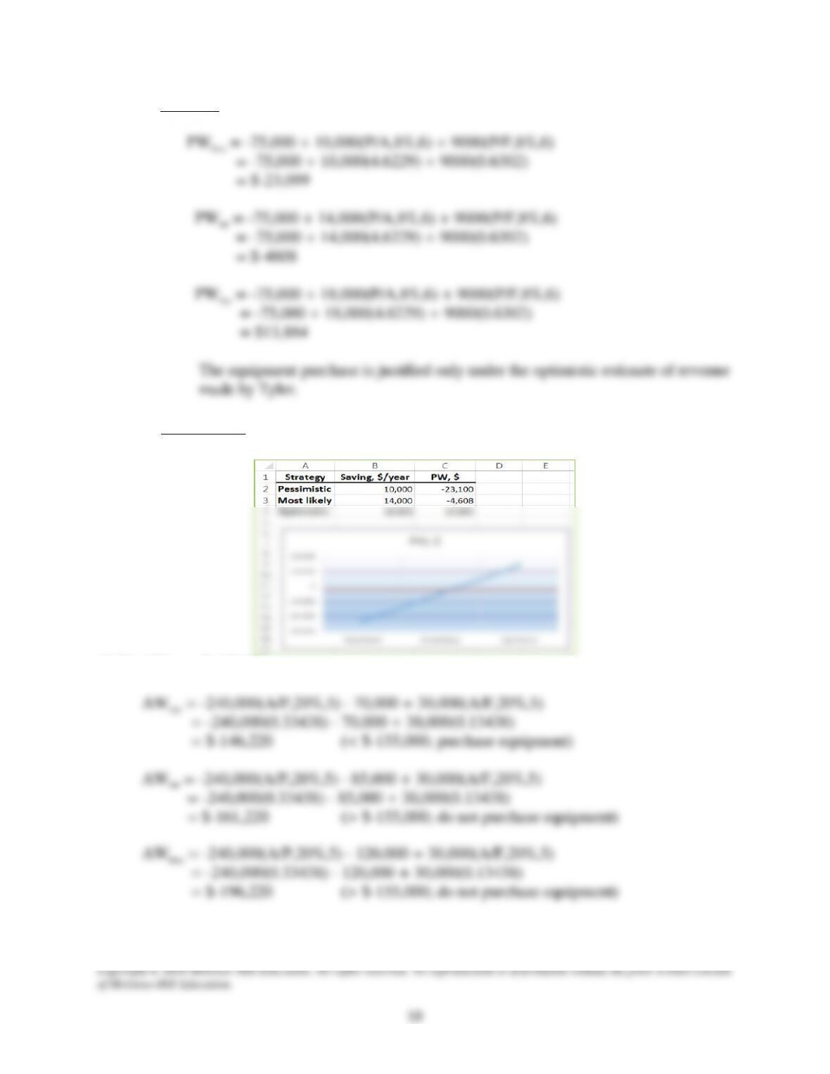
18.20 (a) By hand:
(b) Spreadsheet: Same results. Use the PV function to display the PW values.
18.21 AWcont = $-155,000
Optimistic estimate favors purchase; most likely and pessimistic estimates do not.
Copyright © 2018 McGraw–Hill Education. All rights reserved. No reproduction or distribution without the prior written consent
of McGraw–Hill Education.
11
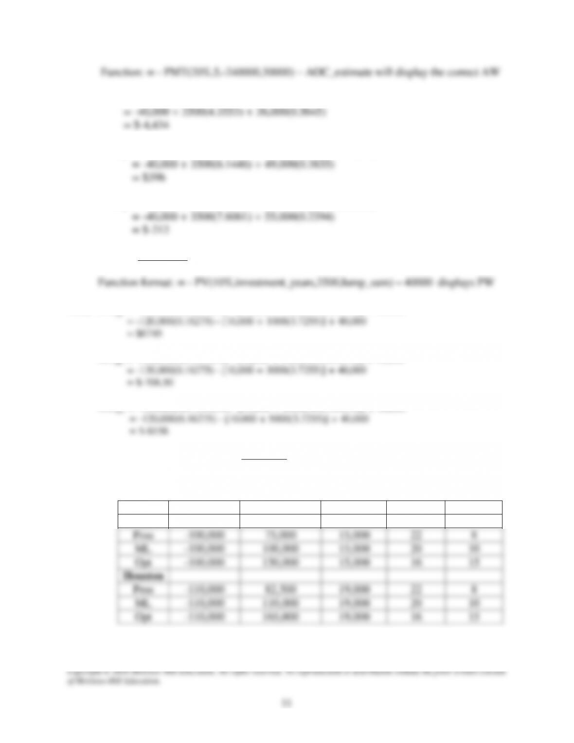
Function: = – PMT(20%,5,-240000,30000) – AOC_estimate will display the correct AW
18.22 PW6 = -40,000 + 3500(P/A,10%,6) + 36,000(P/F,10%,6)
PW10 = -40,000 + 3500(P/A,10%,10) + 49,000(P/F,10%,10)
PW15 = –40,000 + 3500(P/A,10%,15) + 55,000(P/F,10%,15)
The PW is sensitive to the investment period; invest for 10 years
18.23 AWOpt = -120,000(A/P,10%,10) – [10,000 + 1000(A/G,10%,10)] + 40,000
AWML = -120,000(A/P,10%,10) – [10,000 + 3000(A/G,10%,10)] + 40,000
AWPess = -120,000(A/P,10%,10) – [10,000 + 5000(A/G,10%,10)] + 40,000
The decision to expand the BIM is sensitive to gradient increases.
18.24 (a) Tabulated estimates
Location
Investment, $
Market value, $
NCF, $/year
Life, years
MARR, %
Miami
Pess
-100,000
75,000
15,000
22
8
ML
-100,000
100,000
15,000
20
10
Opt
-100,000
150,000
15,000
16
15
Houston
Pess
-110,000
82,500
19,000
22
8
ML
-110,000
110,000
19,000
20
10
Opt
-110,000
165,000
19,000
16
15
(b) Calculations use the PV function. Plots are for MARR, life and market values in table
above.
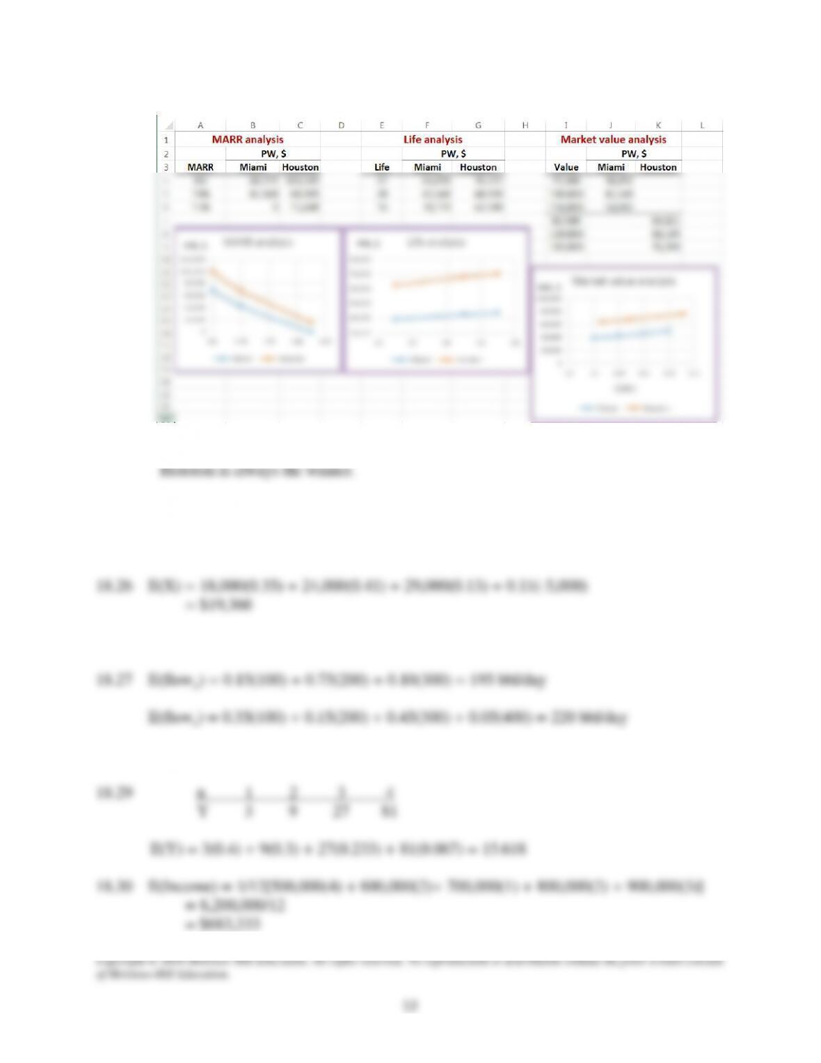
(c) Observing the PW values, Miami always has a lower PW value, so it is not acceptable;
Expected Value
18.25 E(time) = (0.35)(10 + 20) + 0.15(30 + 70) = 25.5 seconds
18.28 E(FW) = 0.15(200,000 – 25,000) + 0.7(40,000) = $54,250