412 CHAPTER 8
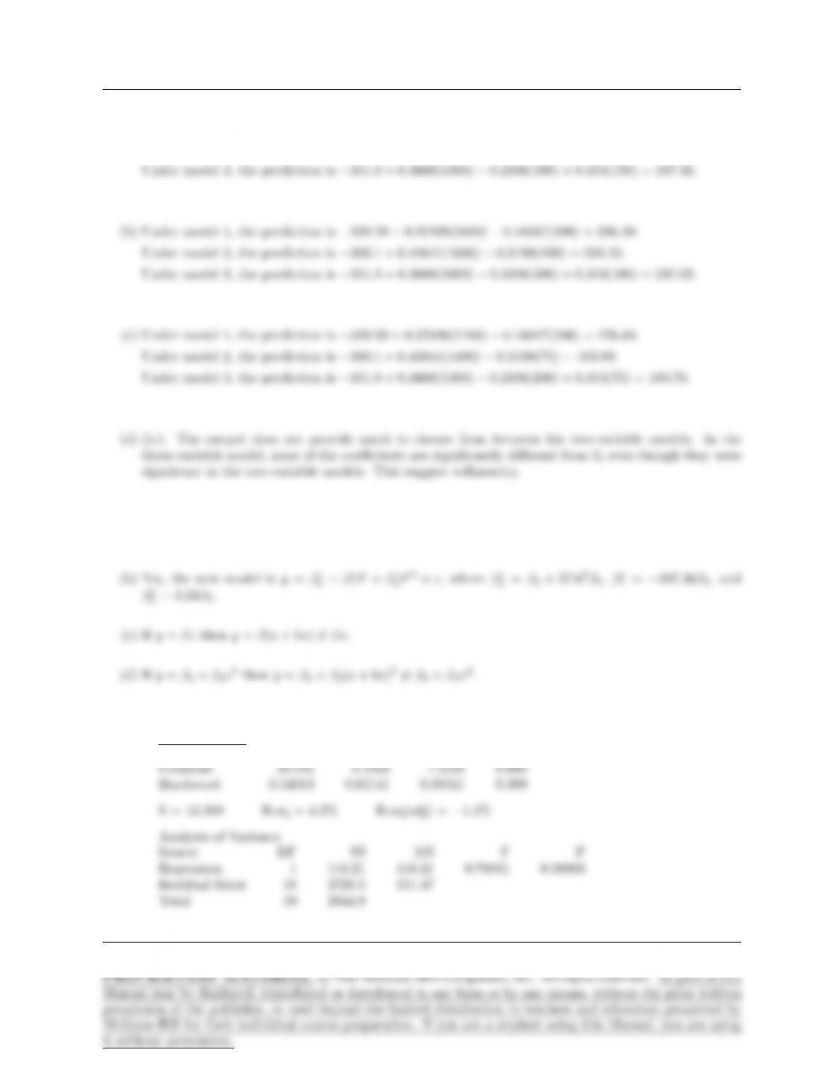
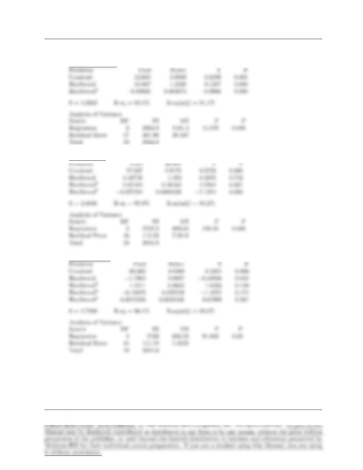
S = 0.33050 R-sq = 92.0% R-sq(adj) = 90.7%
(c)
6 7 8 9 10 11
−1
−0.5
0
0.5
1
Fitted Value
Residual
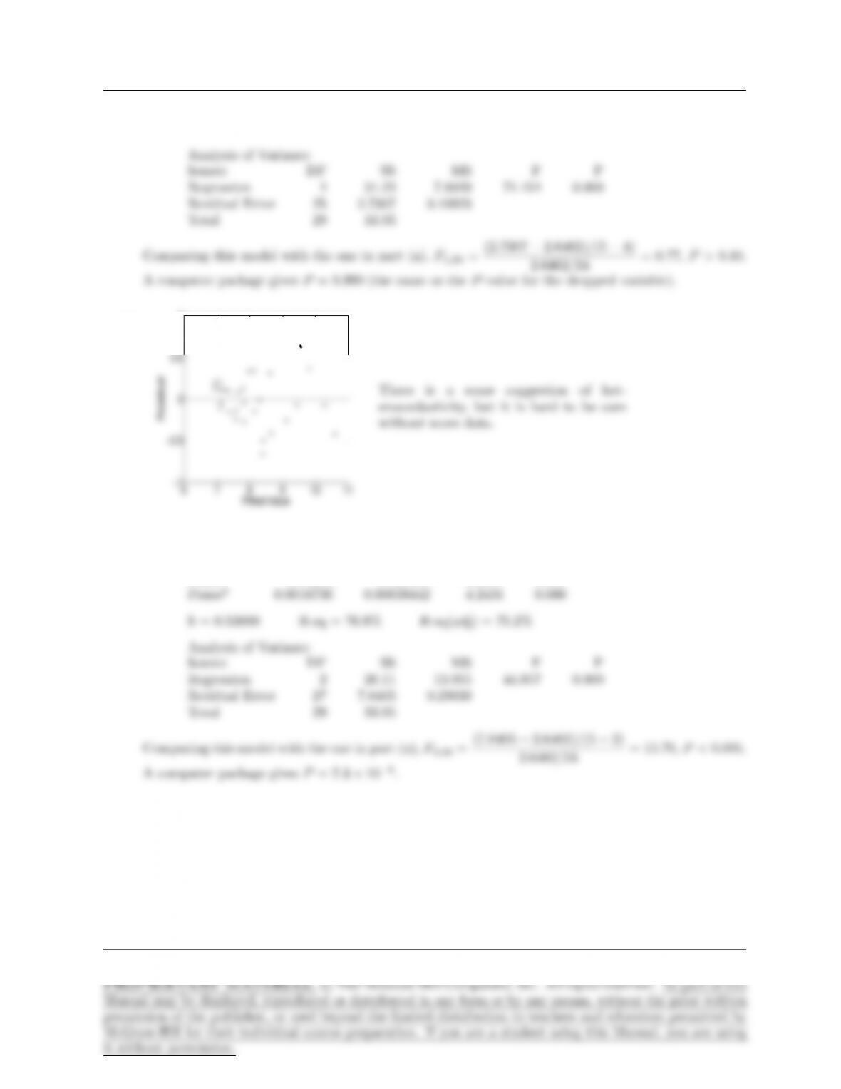
There is a some suggestion of het-
eroscedasticity, but it is hard to be sure
without more data.
(d)
Predictor Coef StDev T P
Constant 9.9601 0.21842 45.601 0.000
Pause -0.13253 0.020545 -6.4507 0.000
Page 412
SUPPLEMENTARY EXERCISES FOR CHAPTER 8 413
(e)
e s d e s
Vars R-Sq R-Sq(adj) C-p S d e 2 2 e
1 61.5 60.1 92.5 0.68318 X
1 60.0 58.6 97.0 0.69600 X
(b) We drop x1:
Predictor Coef StDev T P
414 CHAPTER 8
7.
100 200 300 400
−80
−60
−40
−20
0
20
40
60
80
Linear Model
Fitted Value
Residual
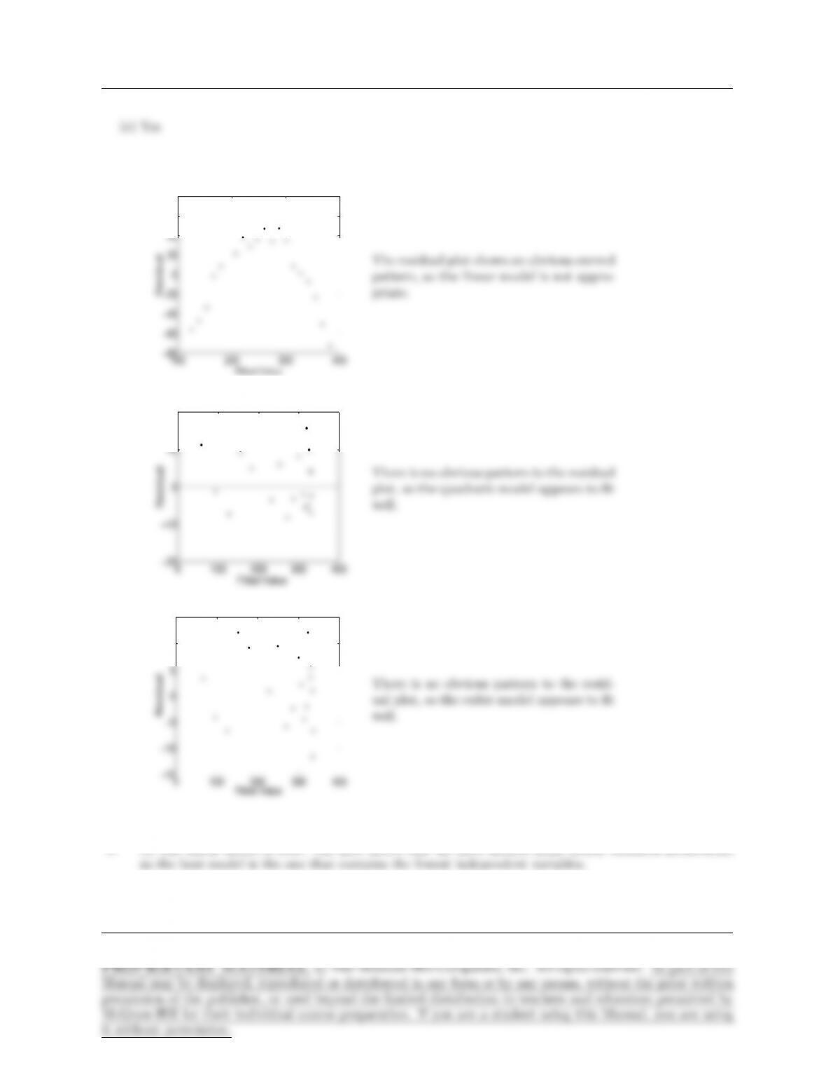
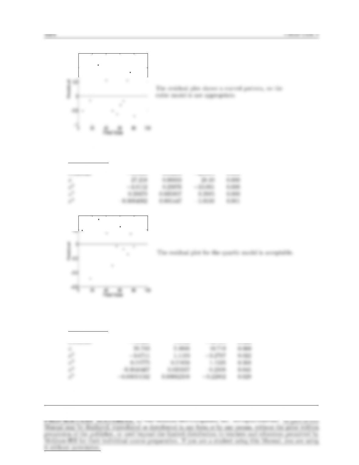
The residual plot shows an obvious curved
pattern, so the linear model is not appro-
priate.
0 100 200 300 400
−20
−10
0
10
20
Quadratic Model
Fitted Value
Residual
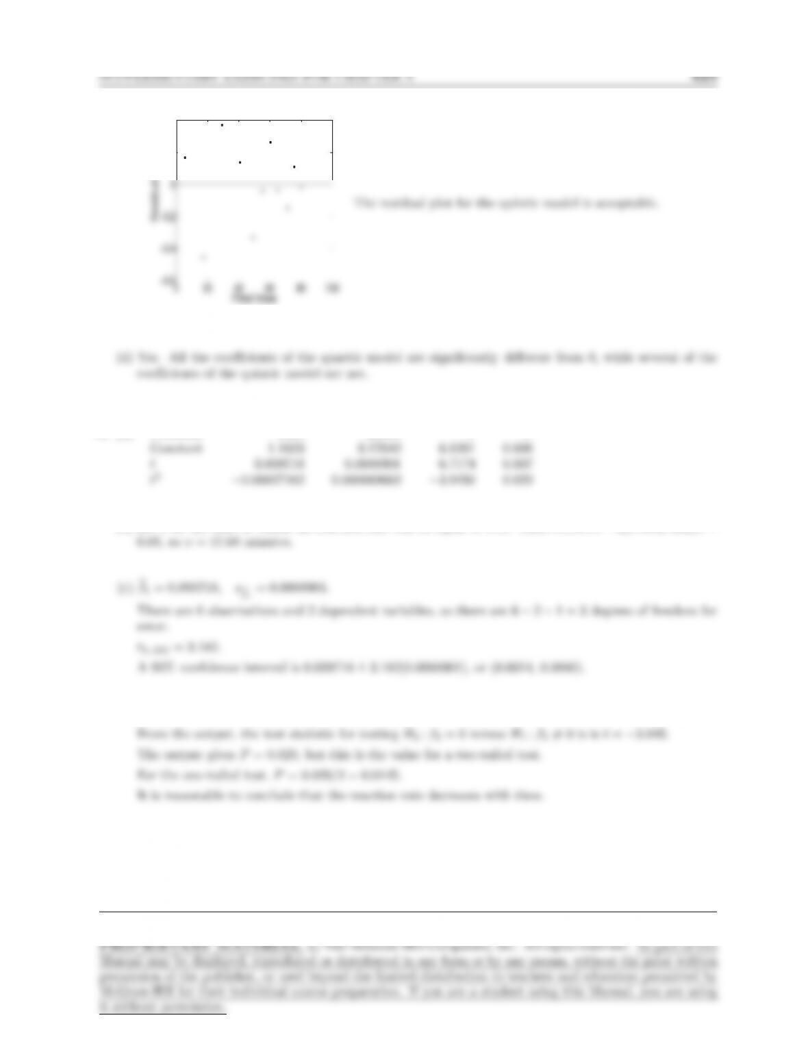
There is no obvious pattern to the residual
plot, so the quadratic model appears to fit
well.
0 100 200 300 400
−15
−10
−5
0
5
10
15
Cubic Model
Fitted Value
Residual
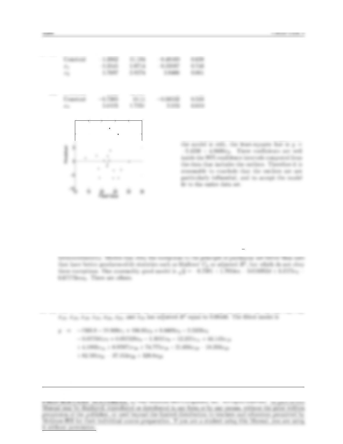
There is no obvious pattern to the resid-
ual plot, so the cubic model appears to fit
well.
8. (i) The linear model is best. The plot shows that all three models make nearly identical predictions,
Page 414
SUPPLEMENTARY EXERCISES FOR CHAPTER 8 415
9. (a) Under model 1, the prediction is −320.59 + 0.37820(1500) −0.16047(400) = 182.52.
Under model 2, the prediction is −380.1 + 0.41641(1500) −0.5198(150) = 166.55.
10. (a) Yes, the new model is y=β∗
0+β∗
1F+ε, where β∗
0=−57.6β1and β∗
1= 1.8β1.
11. (a) Linear Model
Predictor Coef StDev T P
Page 415
416 CHAPTER 8
Quadratic Model
Cubic Model
Quartic Model
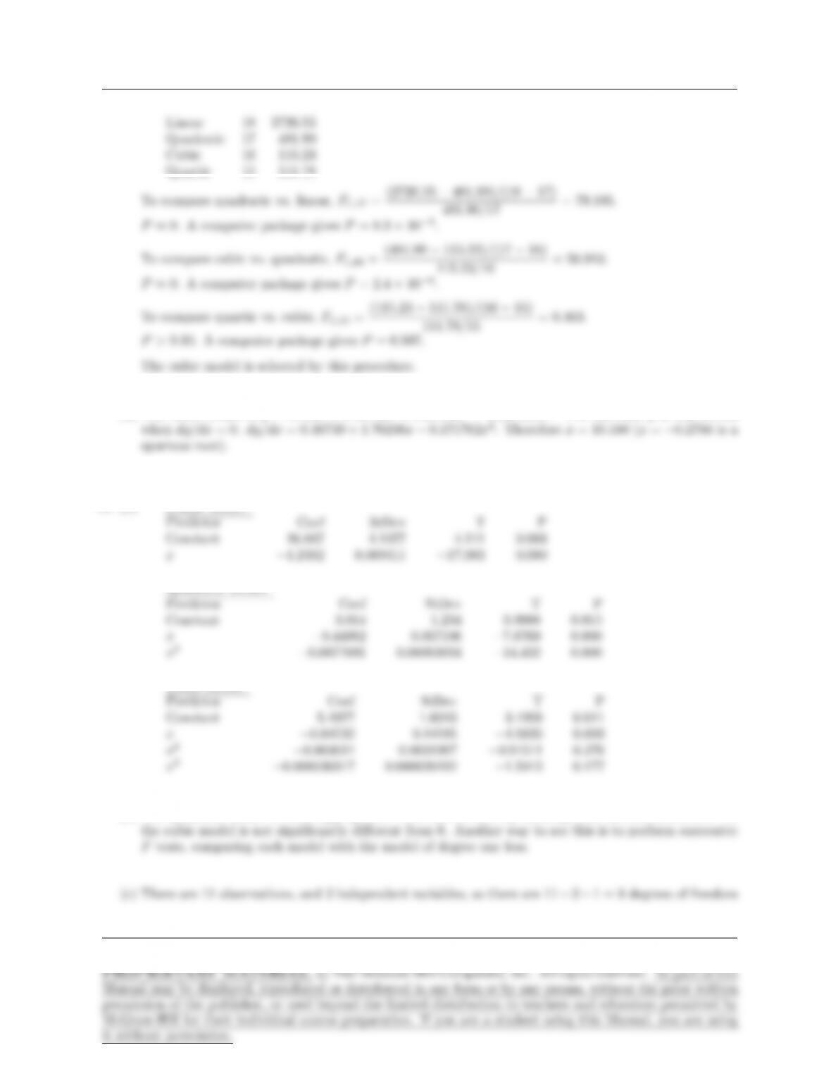
The values of SSE and their degrees of freedom for models of degrees 1, 2, 3, and 4 are:
Page 416
SUPPLEMENTARY EXERCISES FOR CHAPTER 8 417
Quartic 15 111.78
(b) The cubic model is y= 27.937 + 0.48749x+ 0.85104x2−0.057254x3. The estimate yis maximized
12. (a) Linear Model
Quadratic Model
Cubic Model
(b) The quadratic model is most appropriate. This can be seen by noticing that the coefficient of x3in
Page 417
418 CHAPTER 8
13. (a) Let y1represent the lifetime of the sponsor’s paint, y2represent the lifetime of the competitor’s paint,
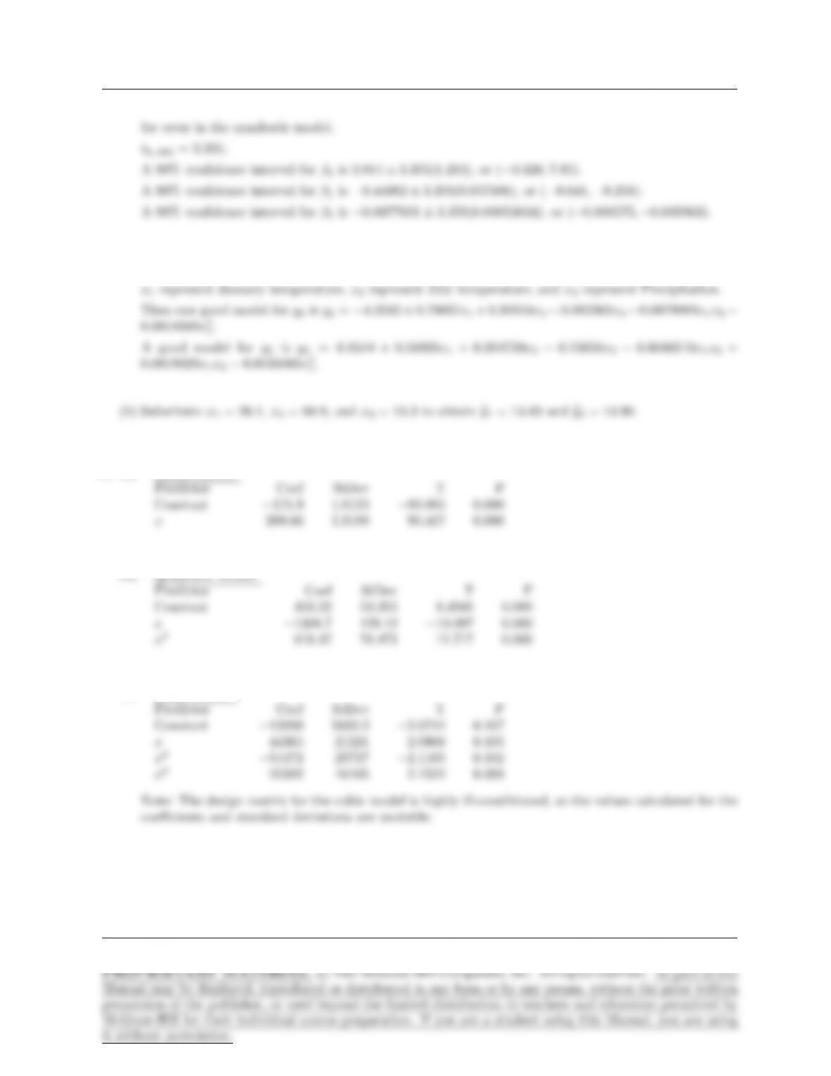
14. (a) Linear Model
(b) Quadratic Model
(c) Cubic Model
(d) The quadratic model. The coefficients are not significant in the cubic model.
Page 418
SUPPLEMENTARY EXERCISES FOR CHAPTER 8 419
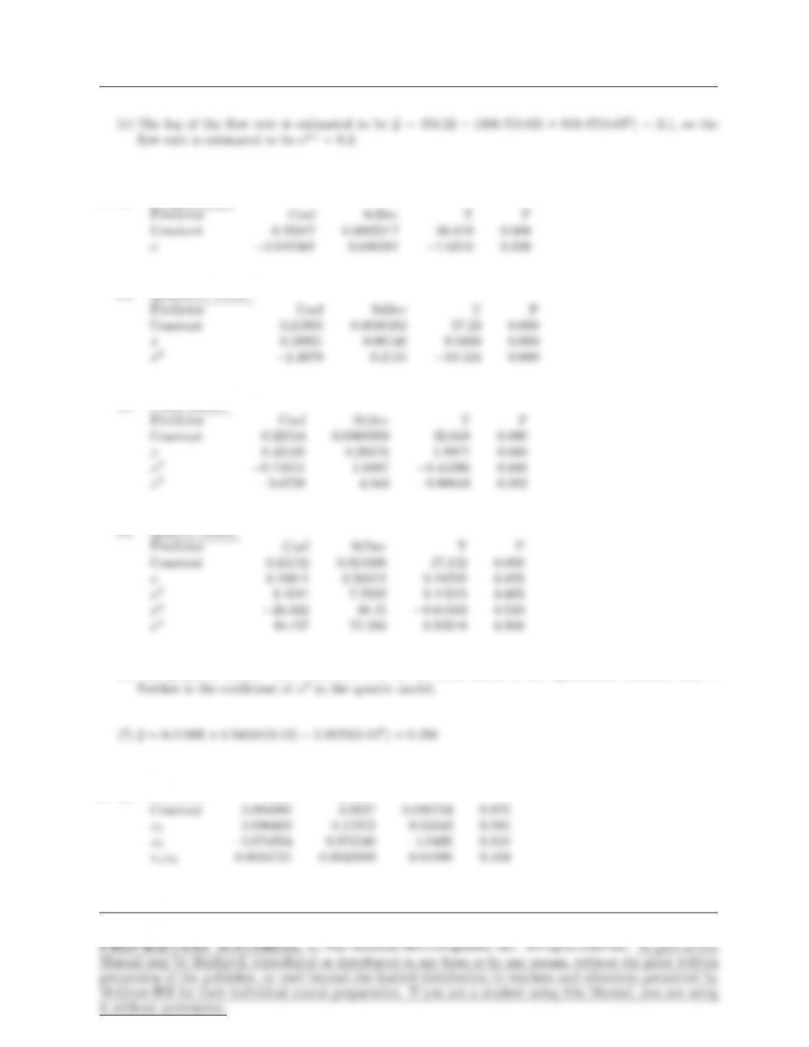
15. (a) Linear Model
(b) Quadratic Model
(c) Cubic Model
(e) The quadratic model. The coefficient of x3in the cubic model is not significantly different from 0.
16. (a) Predictor Coef StDev T P
Page 419
420 CHAPTER 8
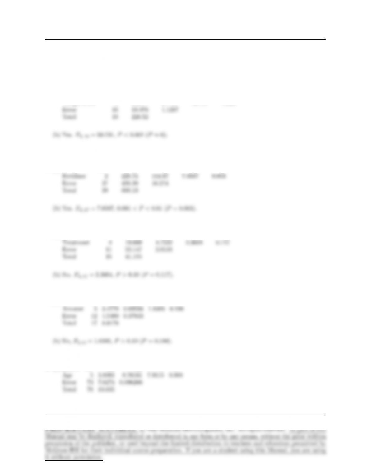
Analysis of Variance
Source DF SS MS F P
(b) Predictor Coef StDev T P
Constant −1.9749 1.7499 −1.1286 0.273
(c) Predictor Coef StDev T P
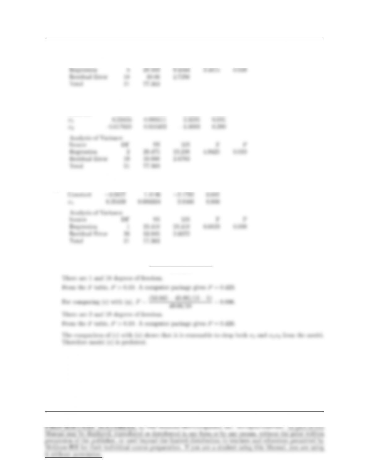
(d) For comparing (b) with (a), F=(50.888 −49.06)/(3 −2)
49.06/18 = 0.671.
Page 420
17. (a) Predictor Coef StDev T P
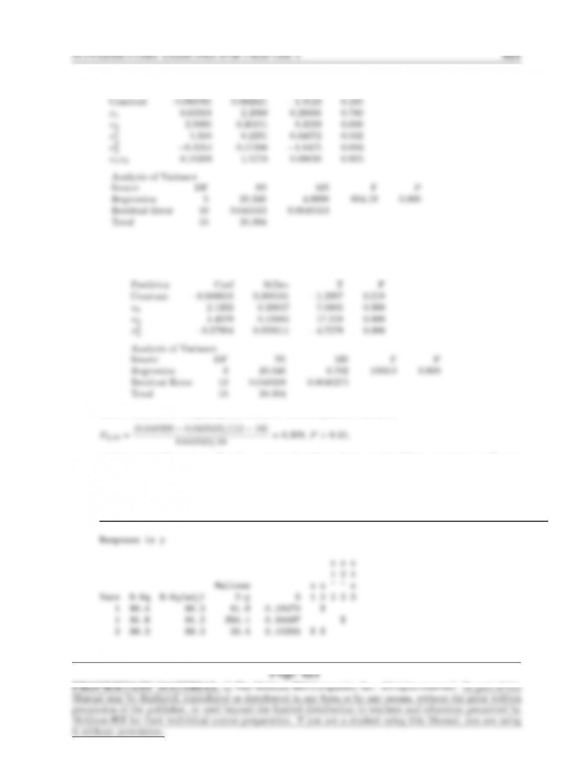
(b) The model containing the variables x1,x2, and x2
2is a good one. Here are the coefficients along with
their standard deviations, followed by the analysis of variance table.
The Fstatistic for comparing this model to the full quadratic model is
so it is reasonable to drop x2
1and x1x2from the full quadratic model. All the remaining coefficients
are significantly different from 0, so it would not be reasonable to reduce the model further.
(c) The output from the MINITAB best subsets procedure is
18. (a) Linear Model
Page 422
SUPPLEMENTARY EXERCISES FOR CHAPTER 8 423
0 20 40 60 80
−2
−1
0
1
2
3
Fitted Value
Residual
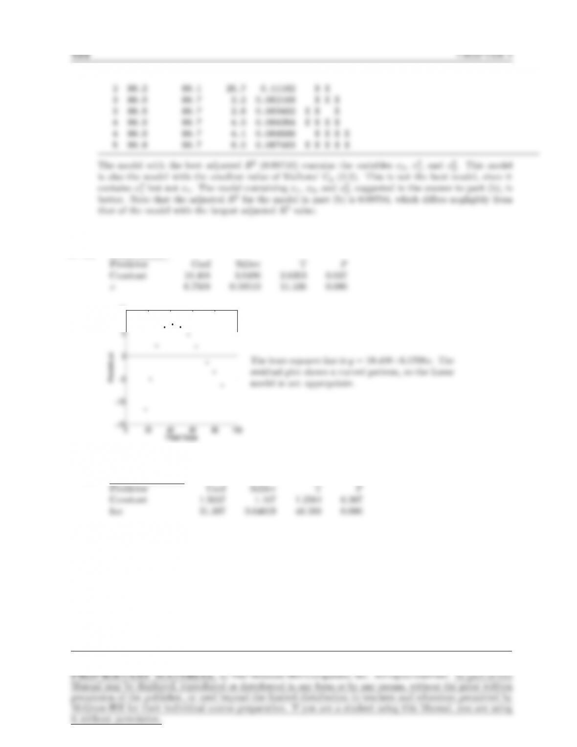
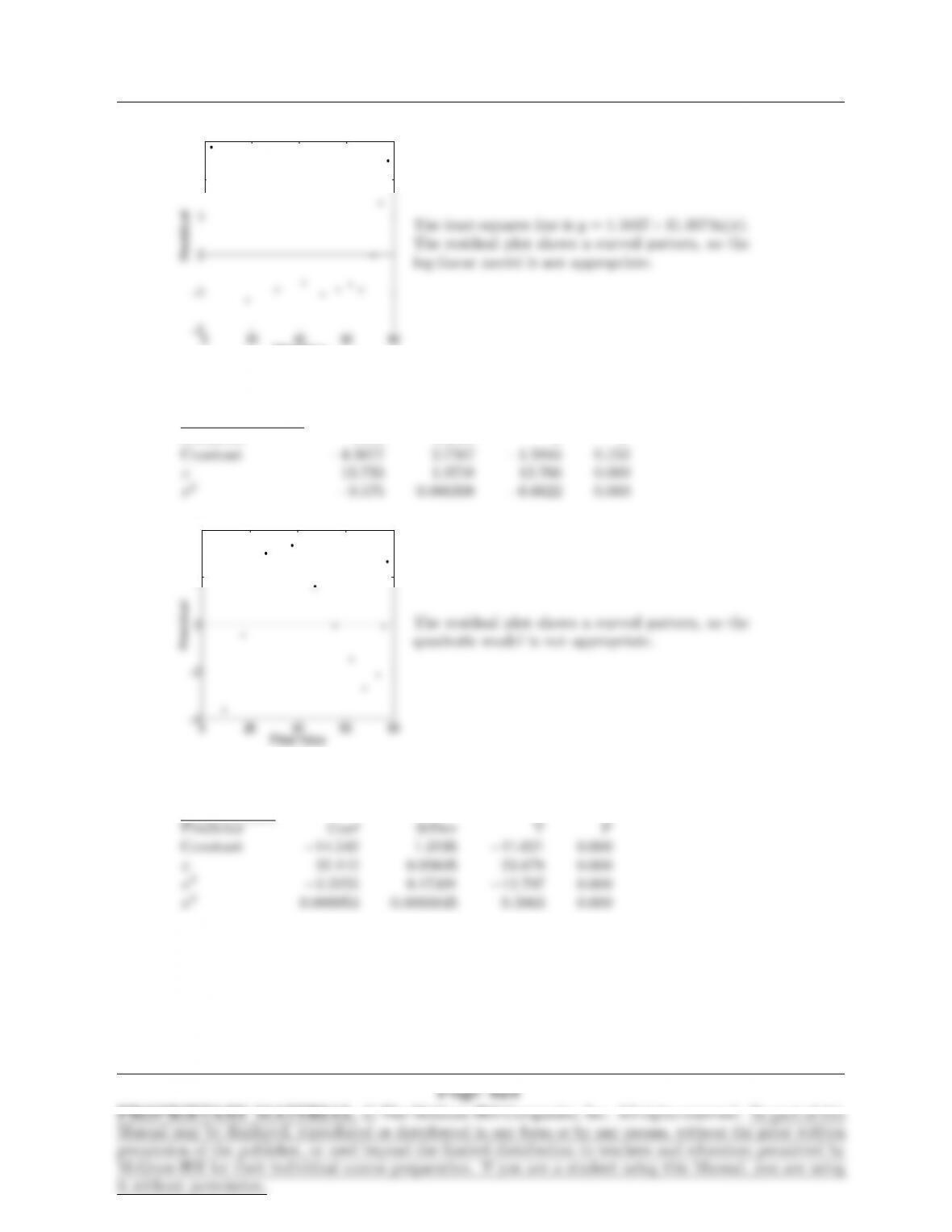
The least-squares line is y= 1.5037+31.397 ln(x).
The residual plot shows a curved pattern, so the
log-linear model is not appropriate.
(c) Quadratic Model
Predictor Coef StDev T P
20. (a) Predictor Coef StDev T P
(b) Predictor Coef StDev T P
(c)
10 15 20 25 30 35
−10
10
15
Fitted Value
The two uppermost points in the plot could be
characterized as outliers. If these are dropped and
21. y=β0+β1x1+β2x2+β3x1x2+ε.
22. There are several good models. The variable yshould be transformed to √yor perhaps ln yto avoid
23. (a) The 17-variable model containing the independent variables x1,x2,x3,x6,x7,x8,x9,x11,x13 ,x14,
Page 426

SUPPLEMENTARY EXERCISES FOR CHAPTER 8 427
(b) The 8-variable model containing the independent variables x1,x2,x5,x8,x10 ,x11,x14 , and x21 has
(e) The 2-variable model z=−1660.9 + 0.67152x7+ 134.28x10 has Mallows’ Cpequal to −4.0.
(f) Using a value of 0.15 for both α-to-enter and α-to-remove, the equation chosen by stepwise regression is
Page 427
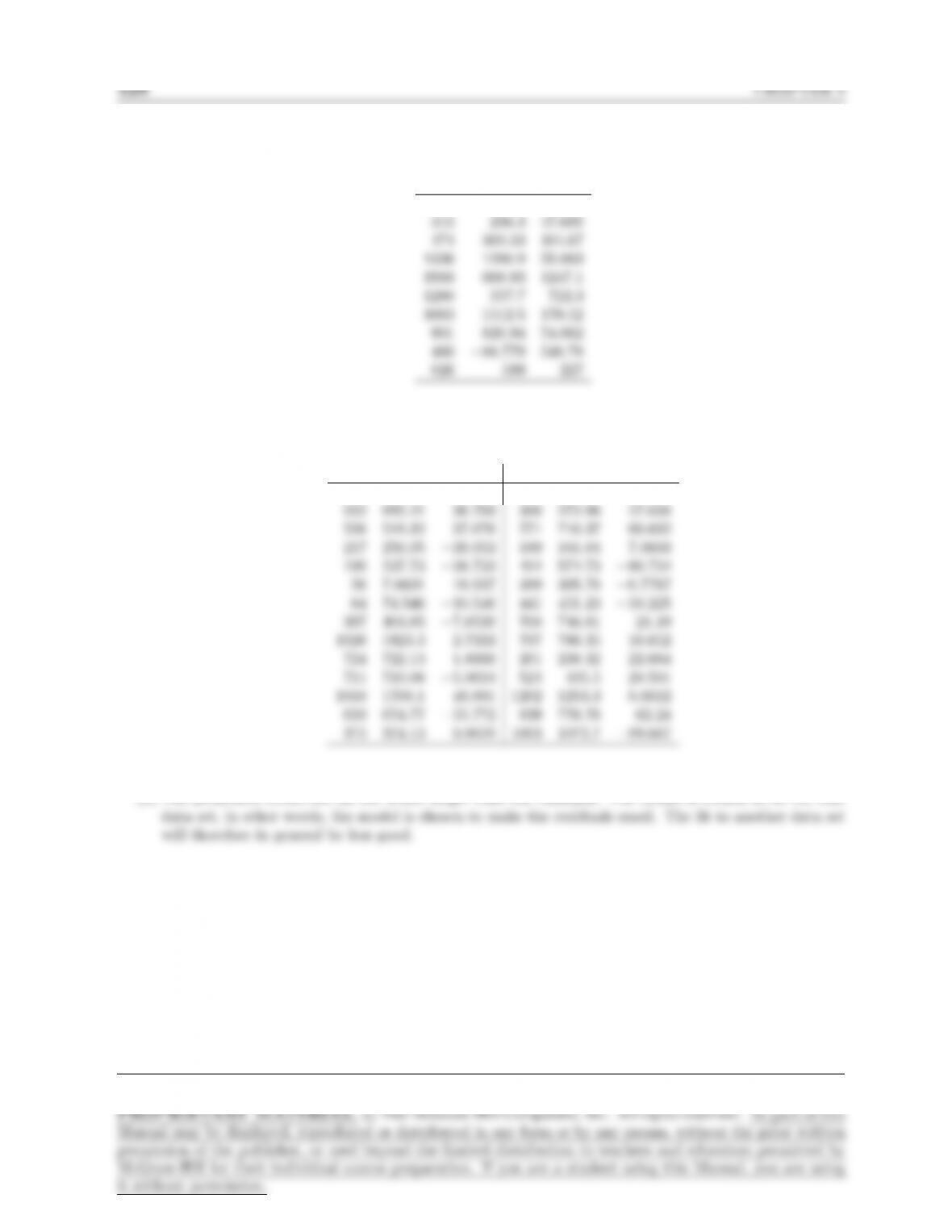
24. (a, b) The predicted values and prediction errors for the new dataset are:
yPred Error
1713 508.99 1204
(c) The fitted values and residuals for the 28 row dataset are:
yFit Resid yFit Resid
1850 1900.3−50.307 214 266.69 −52.693
(d) The prediction errors are on the whole larger than the residuals. The model is chosen to fit the first
Page 428
SECTION 9.1 429
Chapter 9
Section 9.1
1. (a) Source DF SS MS F P
Temperature 3 202.44 67.481 59.731 0.000
2. (a) Source DF SS MS F P
3. (a) Source DF SS MS F P
4. (a) Source DF SS MS F P
5. (a) Source DF SS MS F P
Page 429