5-41
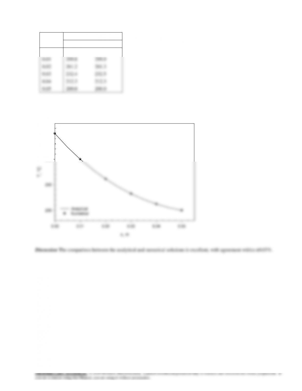
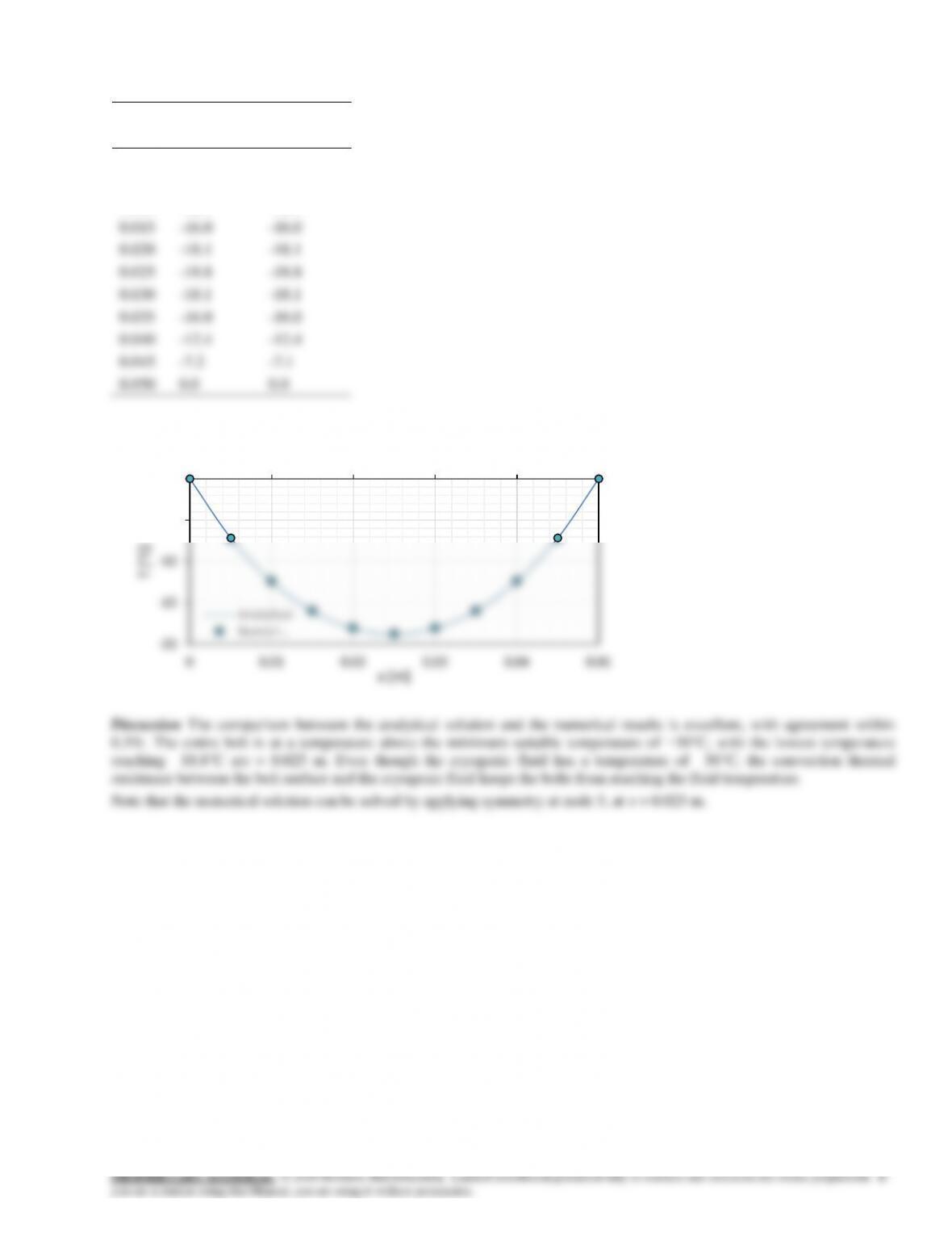
The nodal temperatures for analytical and numerical solutions are tabulated in the following table:
x, m
T(x),°C
Analytical
Numerical
0
350.0
350.0
0.01
299.8
299.9
0.02
261.2
261.3
0.03
232.4
232.5
0.04
212.3
212.3
0.05
200.0
200.0
The comparison of the analytical and numerical solutions is shown in the following figure:
x, m
0.00 0.01 0.02 0.03 0.04 0.05
T, °C
200
250
300
350
Analytical
Numerical
Discussion The comparison between the analytical and numerical solutions is excellent, with agreement within ±0.05%.
5-42
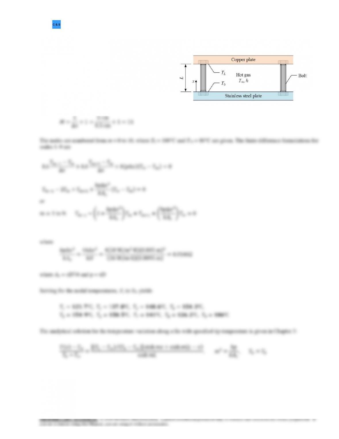
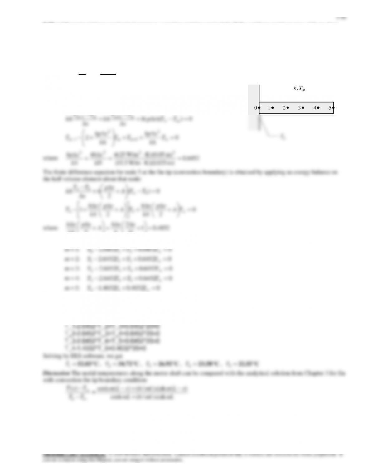
5-48 A stainless steel plate is connected to a copper plate by long ASTM B98 copper-silicon bolts. Portion of the bolts
are exposed to convection with hot gas. The temperatures, T0 at x = 0 and TL at x = L, are known. Determine the nodal
temperatures and compare them with the analytical solution. Would any part of the ASTM B98 bolts be above the maximum
use temperature of 149°C?
Assumptions1 Heat transfer is steady and one
dimensional. 2 The part of the bolt exposed to convection
behaves as finned surface. 3 Thermal properties are
constant. 4 Thermal radiation is neglected.
Properties The thermal conductivity for the bolts is 36
W/m·K.
Analysis The nodal spacing is given as Δx = 5 mm. So,
the number of nodes is
5-43
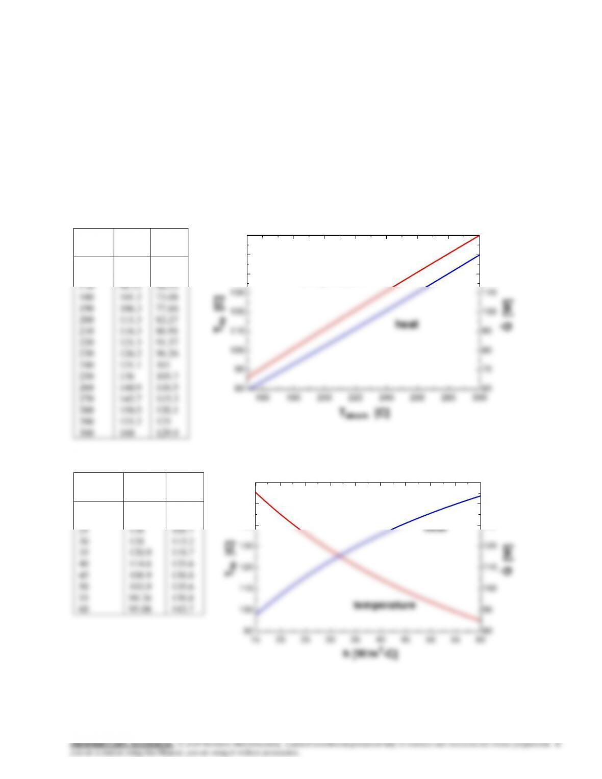
The analytical and numerical results are tabulated in the following table:
Analytical
Numerical
x [m]
T [°C]
T [°C]
0
100.0
100.0
0.005
121.7
121.7
0.010
137.8
137.8
0.015
148.7
148.6
0.020
154.4
154.3
0.025
155.0
154.9
0.030
150.6
150.5
0.035
141.1
141.0
0.040
126.3
126.2
0.045
106.0
106.0
0.050
80.0
80.0
The temperature distribution along the bolt, as a function of x, is plotted in the following figure:
70
90
110
130
150
170
0 0.01 0.02 0.03 0.04 0.05
T [°C]
x [m]
Analy…
Num…
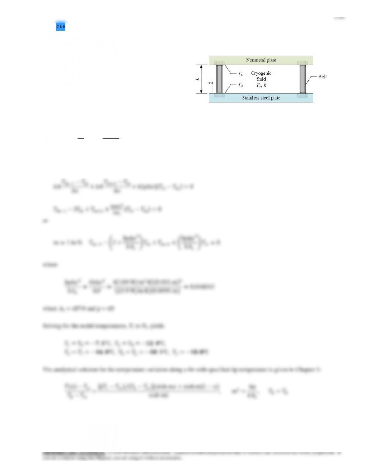
5-45
The analytical and numerical results are tabulated in the following table:
Analytical
Numerical
x [m]
T [°C]
T [°C]
0
0.0
0.0
0.005
-7.2
-7.1
0.010
-12.4
-12.4
0.015
-16.0
-16.0
0.020
-18.1
-18.1
0.025
-18.8
-18.8
0.030
-18.1
-18.1
0.035
-16.0
-16.0
0.040
-12.4
-12.4
0.045
-7.2
-7.1
0.050
0.0
0.0
The temperature distribution along the bolt, as a function of x, is plotted in the following figure:
-20
-15
-10
-5
0
0 0.01 0.02 0.03 0.04 0.05
T [°C]
x [m]
Analytical
Numeri…
5-47
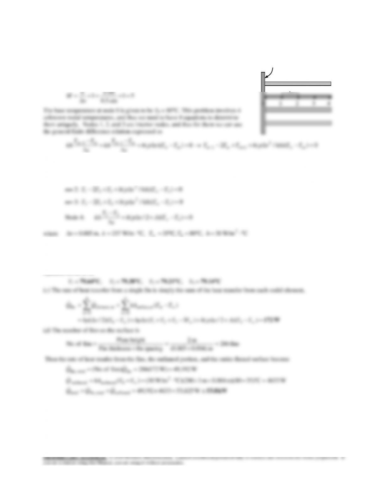
5-51 One side of a hot vertical plate is to be cooled by attaching aluminum fins of rectangular profile. The finite difference
formulation of the problem for all nodes is to be obtained, and the nodal temperatures, the rate of heat transfer from a single
fin and from the entire surface of the plate are to be determined.
Assumptions 1 Heat transfer along the fin is given to be steady and one-dimensional. 2 The thermal conductivity is constant.
3 Combined convection and radiation heat transfer coefficient is constant and uniform.
Properties The thermal conductivity is given to be k = 237 W/m°C.
Analysis (a) The nodal spacing is given to be x=0.5 cm. Then the
number of nodes M becomes
cm 2
L
x
x
The finite difference equation for node 4 at the fin tip is obtained by applying an energy
balance on the half volume element about that node. Then,
m= 1:
0))(/(2 1
2
210 =−++− TTkAxphTTT
2
and
m 006.6)m 003.03(2 and m 0.009m) m)(0.003 3( 2=+=== pA
.
This system of 4 equations with 4 unknowns constitute the finite difference formulation of the problem.
(b) The nodal temperatures under steady conditions are determined by solving the 4 equations above simultaneously with an
equation solver to be
kW 53.8=+=+=
W53,8254633192,49
unfinned totalfin,total
QQQ
T0
h, T
x
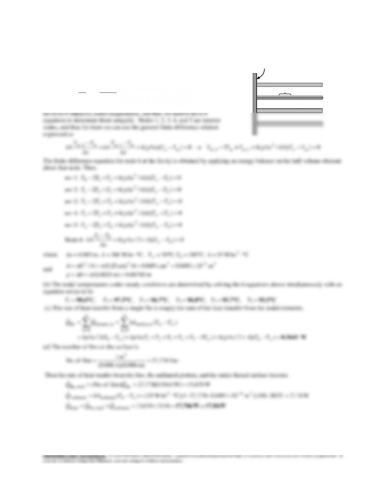
5-49
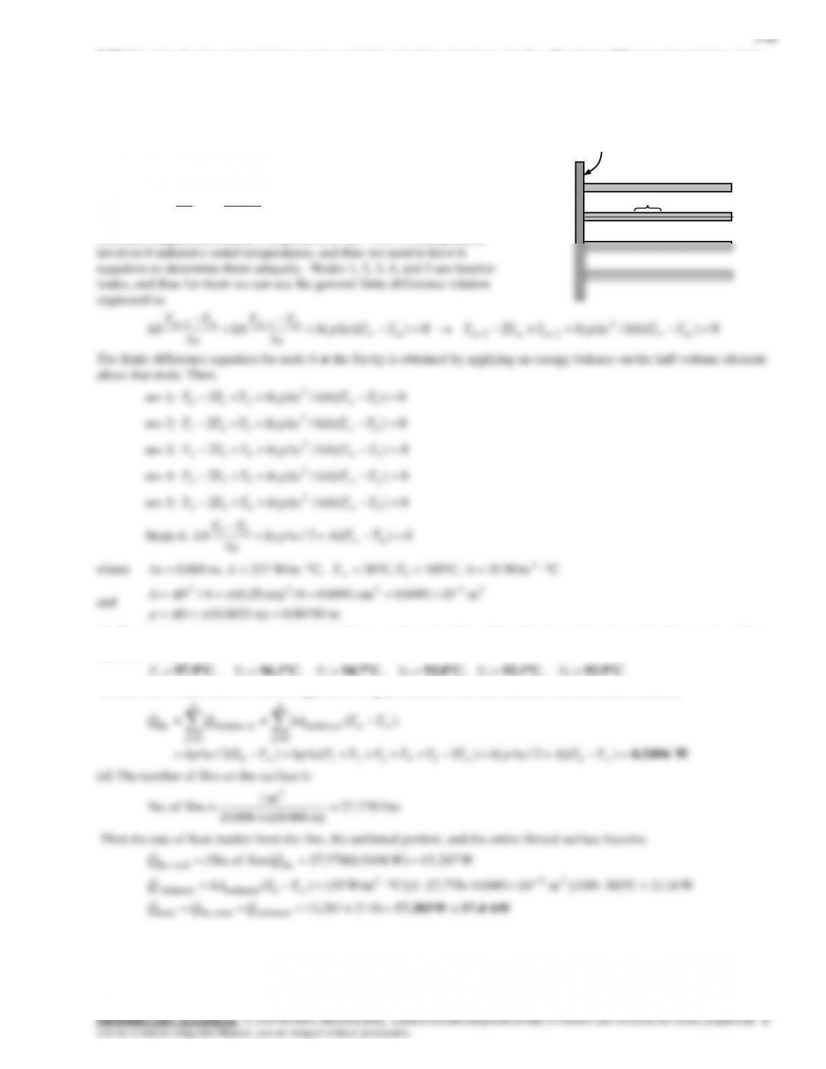
5-53 One side of a hot vertical plate is to be cooled by attaching copper pin fins. The finite difference formulation of the
problem for all nodes is to be obtained, and the nodal temperatures, the rate of heat transfer from a single fin and from the
entire surface of the plate are to be determined.
Assumptions 1 Heat transfer along the fin is given to be steady and one-dimensional. 2 The thermal conductivity is constant.
3 Combined convection and radiation heat transfer coefficient is constant and uniform.
Properties The thermal conductivity is given to be k = 386 W/m°C.
Analysis (a) The nodal spacing is given to be x=0.5 cm. Then the number
of nodes M becomes
71
cm 5.0
cm 3
1=+=+
=x
L
M
The base temperature at node 0 is given to be T0 = 100C. This problem
kW 17.8 W17,786 =+=+=
2116670,15
unfinned totalfin,total
QQQ
T0
h, T
x
• • • • • • •
0 1 2 3 4 5 6
5-50
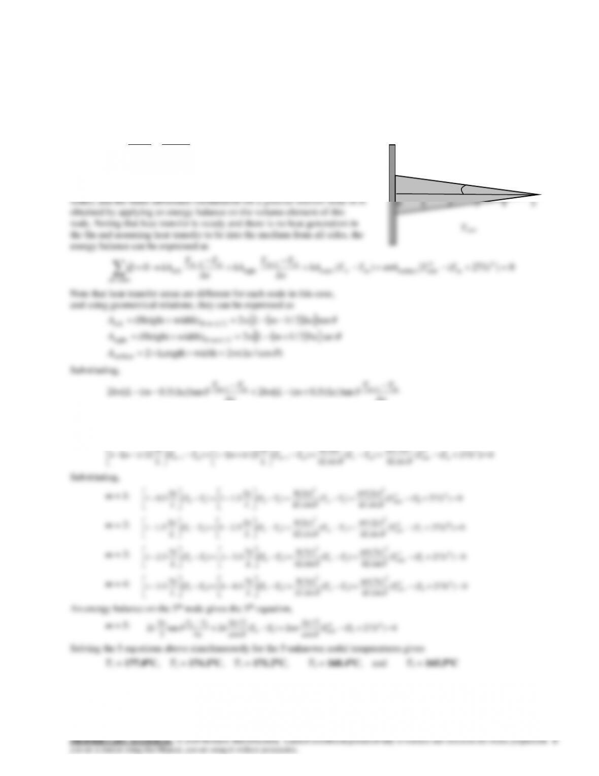
5-54 A long triangular fin attached to a surface is considered. The nodal temperatures, the rate of heat transfer, and the fin
efficiency are to be determined numerically using 6 equally spaced nodes.
Assumptions 1 Heat transfer along the fin is given to be steady, and the temperature along the fin to vary in the x direction
only so that T = T(x). 2 Thermal conductivity is constant.
Properties The thermal conductivity is given to be k = 180 W/m°C. The emissivity of the fin surface is 0.9.
Analysis The fin length is given to be L = 5 cm, and the number of nodes is specified to be M = 6. Therefore, the nodal
spacing x is
m 01.0
1–6
m 05.0
1==
−
= M
L
x
The temperature at node 0 is given to be T0 = 180°C, and the temperatures
at the remaining 5 nodes are to be determined. Therefore, we need to have 5
equations to determine them uniquely. Nodes 1, 2, 3, and 4 are interior
0]})273([)(){cos/(2
tan])5.0([2tan])5.0([2
44
surr
11
=+−+−+
−
+−+
−
−−
+−
mm
mmmm
TTTThxw
x
TT
xmLkw
x
TT
xmLkw
Dividing each term by
tan2kwL
/x gives
( ) ( )
0])273([
sin
)(
)(
sin
)(
)(2/11)(2/11 44
surr
22
11 =+−
+−
+−
+−+−
−− +− mmmmmm TT
kL
x
TT
kL
xh
TT
L
x
mTT
L
x
m
Substituting,
m = 1:
0])273([
sin
)(
)(
sin
)(
)(5.11)(5.01 4
1
4
surr
2
1
2
1210 =+−
+−
+−
−+−
−TT
kL
x
TT
kL
xh
TT
L
x
TT
L
x
m = 2:
0])273([
sin
)(
)(
sin
)(
)(5.21)(5.11 4
2
4
surr
2
2
2
2321 =+−
+−
+−
−+−
−TT
kL
x
TT
kL
xh
TT
L
x
TT
L
x
m = 3:
0])273([
sin
)(
)(
sin
)(
)(5.31)(5.21 4
3
4
surr
2
3
2
3432 =+−
+−
+−
−+−
−TT
kL
x
TT
kL
xh
TT
L
x
TT
L
x
m = 4:
0])273([
sin
)(
)(
sin
)(
)(5.41)(5.31 4
4
4
surr
2
4
2
4543 =+−
+−
+−
−+−
−TT
kL
x
TT
kL
xh
TT
L
x
TT
L
x
An energy balance on the 5th node gives the 5th equation,
m = 5:
0])273([
cos
2/
2)(
cos
2/
2tan
2
24
5
4
surr5
54 =+−
+−
+
−
TT
x
TT
x
h
x
TTx
k
Solving the 5 equations above simultaneously for the 5 unknown nodal temperatures gives
T1 = 177.0C, T2 = 174.1C, T3 = 171.2C, T4 = 168.4C, and T5 = 165.5C
T0
h, T
•
•
•
•
•
•
x
5-51
(b) The total rate of heat transfer from the fin is simply the sum of the heat transfer from each volume element to the ambient,
and for w = 1 m it is determined from
4
5
5
5

5-52
5-55 Prob. 5-54 is reconsidered. The effect of the fin base temperature on the fin tip temperature and the rate of heat
transfer from the fin is to be investigated.
Analysis The problem is solved using EES, and the solution is given below.
“GIVEN”
k=180 [W/m-C]
L=0.05 [m]
b=0.01 [m]
w=1 [m]
T_0=180 [C]
T_infinity=25 [C]
h=25 [W/m^2-C]
T_surr=290 [K]
M=6
epsilon=0.9
tan(theta)=(0.5*b)/L
sigma=5.67E-8 [W/m^2-K^4] “Stefan-Boltzmann constant”
“ANALYSIS”
“(a)”
DELTAx=L/(M-1)
“Using the finite difference method, the five equations for the temperatures at 5 nodes are determined to be”
(1-0.5*DELTAx/L)*(T_0-T_1)+(1-1.5*DELTAx/L)*(T_2-T_1)+(h*DELTAx^2)/(k*L*sin(theta))*(T_infinity–
T_1)+(epsilon*sigma*DELTAX^2)/(k*L*sin(theta))*(T_surr^4–(T_1+273)^4)=0 “for mode 1″
(1-1.5*DELTAx/L)*(T_1-T_2)+(1-2.5*DELTAx/L)*(T_3-T_2)+(h*DELTAx^2)/(k*L*sin(theta))*(T_infinity–
T_2)+(epsilon*sigma*DELTAX^2)/(k*L*sin(theta))*(T_surr^4–(T_2+273)^4)=0 “for mode 2″
(1-2.5*DELTAx/L)*(T_2-T_3)+(1-3.5*DELTAx/L)*(T_4-T_3)+(h*DELTAx^2)/(k*L*sin(theta))*(T_infinity–
T_3)+(epsilon*sigma*DELTAX^2)/(k*L*sin(theta))*(T_surr^4–(T_3+273)^4)=0 “for mode 3″
(1-3.5*DELTAx/L)*(T_3-T_4)+(1-4.5*DELTAx/L)*(T_5-T_4)+(h*DELTAx^2)/(k*L*sin(theta))*(T_infinity–
T_4)+(epsilon*sigma*DELTAX^2)/(k*L*sin(theta))*(T_surr^4-(T_4+273)^4)=0 “for mode 4″
2*k*DELTAx/2*tan(theta)*(T_4-T_5)/DELTAx+2*h*(0.5*DELTAx)/cos(theta)*(T_infinity–
T_5)+2*epsilon*sigma*(0.5*DELTAx)/cos(theta)*(T_surr^4-(T_5+273)^4)=0 “for mode 5”
T_tip=T_5
“(b)”
Q_dot_fin=C+D “where”
C=h*(w*DELTAx)/cos(theta)*((T_0-T_infinity)+2*(T_1-T_infinity)+2*(T_2-T_infinity)+2*(T_3-T_infinity)+2*(T_4–
T_infinity)+(T_5-T_infinity))
D=epsilon*sigma*(w*DELTAx)/cos(theta)*(((T_0+273)^4-T_surr^4)+2*((T_1+273)^4-T_surr^4)+2*((T_2+273)^4–
T_surr^4)+2*((T_3+273)^4-T_surr^4)+2*((T_4+273)^4-T_surr^4)+((T_5+273)^4-T_surr^4))
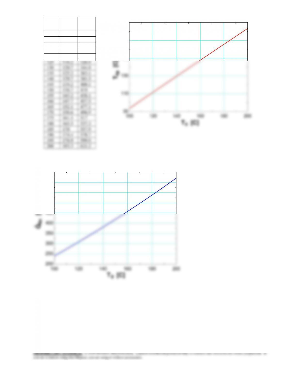
5-53
T0
[C]
Ttip
[C]
fin
Q
[W]
100
93.51
239.8
105
98.05
256.8
110
102.6
274
115
107.1
291.4
120
111.6
309
125
116.2
326.8
130
120.7
344.8
135
125.2
363.1
140
129.7
381.5
145
134.2
400.1
150
138.7
419
155
143.2
438.1
160
147.7
457.5
165
152.1
477.1
170
156.6
496.9
175
161.1
517
180
165.5
537.3
185
170
557.9
190
174.4
578.7
195
178.9
599.9
200
183.3
621.2
100 120 140 160 180 200
90
110
130
150
170
190
T0 [C]
Ttip [C]
5-54
5-56 Two cast iron steam pipes are connected to each other through two 1-cm thick flanges, and heat is lost from the flanges
by convection and radiation. The finite difference formulation of the problem for all nodes is to be obtained, and the
temperature of the tip of the flange as well as the rate of heat transfer from the exposed surfaces of the flange are to be
determined.
Assumptions 1 Heat transfer through the flange is stated to be steady and
one-dimensional. 2 The thermal conductivity and emissivity are constants.
3 Convection heat transfer coefficient is constant and uniform.
PropertiesThe thermal conductivity and emissivity are given to be k = 52
W/m°C and = 0.8.
Analysis(a) The distance between nodes 0 and 1 is the thickness of the
pipe, x1=0.4 cm=0.004 m. The nodal spacing along the flange is given to
be x2=1 cm = 0.01 m. Then the number of nodes M becomes
72
cm 1
cm 5
2=+=+
=x
L
M
hi
Ti
x
•••••••
0 1 2 3 4 5 6
ho, T
Tsurr

5-56
“(c)”
Q_dot=Q_dot_1+Q_dot_2+Q_dot_3+Q_dot_4+Q_dot_5+Q_dot_6 “where”
Q_dot_1=h*2*2*pi*t*(r_1+r_12)/2*DELTAx_2/2*(T_1–
T_infinity)+epsilon*sigma*2*2*pi*t*(r_1+r_12)/2*DELTAx_2/2*((T_1+273)^4–T_surr^4)
Q_dot_2=h*2*2*pi*t*r_2*DELTAx_2*(T_2-T_infinity)+epsilon*sigma*2*2*pi*t*r_2*DELTAx_2*((T_2+273)^4–
T_surr^4)
Q_dot_3=h*2*2*pi*t*r_3*DELTAx_2*(T_3-T_infinity)+epsilon*sigma*2*2*pi*t*r_3*DELTAx_2*((T_3+273)^4–
T_surr^4)
Q_dot_4=h*2*2*pi*t*r_4*DELTAx_2*(T_4-T_infinity)+epsilon*sigma*2*2*pi*t*r_4*DELTAx_2*((T_4+273)^4–
T_surr^4)
Q_dot_5=h*2*2*pi*t*r_5*DELTAx_2*(T_5-T_infinity)+epsilon*sigma*2*2*pi*t*r_5*DELTAx_2*((T_5+273)^4–
T_surr^4)
Q_dot_6=h*2*(2*pi*t*(r_56+r_6)/2*(DELTAx_2/2)+2*pi*t*r_6)*(T_6–
T_infinity)+epsilon*sigma*2*(2*pi*t*(r_56+r_6)/2*(DELTAx_2/2)+2*pi*t*r_6)*((T_6+273)^4-T_surr^4)
Tsteam
[C]
Ttip
[C]
Q
[W]
150
160
170
180
190
200
210
220
230
240
250
260
270
280
290
300
85.87
91.01
96.12
101.2
106.3
111.3
116.3
121.3
126.2
131.1
136
140.9
145.7
150.5
155.2
160
59.48
63.99
68.52
73.08
77.66
82.27
86.91
91.57
96.26
101
105.7
110.5
115.3
120.1
125
129.9
h
[W/m2.C]
Ttip
[C]
Q
[W]
15
20
25
30
35
40
45
50
55
60
155.4
145.1
136
128
120.9
114.6
108.9
103.9
99.26
95.08
87.7
97.31
105.7
113.2
119.7
125.6
130.8
135.6
139.8
143.7
160 180 200 220 240 260 280 300
80
90
100
110
120
130
140
150
160
60
70
80
90
100
110
120
130
140
Tsteam [C]
Ttip [C]
Q [W]
temperature
heat
100
110
120
130
140
150
160
90
100
110
120
130
140
150
Ttip [C]
Q [W]
temperature
heat

5-58
5-60 Using EES, the solutions of the systems of algebraic equations are determined to be as follows:
“(a)”
4*x_1-x_2+2*x_3+x_4=-6
x_1+3*x_2-x_3+4*x_4=-1
-x_1+2*x_2+5*x_4=5
2*x_2-4*x_3-3*x_4=-5
“(b)”
2*x_1+x_2^4-2*x_3+x_4=1
x_1^2+4*x_2+2*x_3^2-2*x_4=-3
-x_1+x_2^4+5*x_3=10
3*x_1-x_3^2+8*x_4=15
5-59
Two–Dimensional Steady Heat Conduction
5-62C For a medium in which the finite difference formulation of a general interior node is given in its simplest form as
4/)( bottomrighttopleftnode TTTTT +++=
:
(a) Heat transfer is steady, (b) heat transfer is two-dimensional, (c) there is no heat generation in the medium, (d) the nodal
spacing is constant, and (e) the thermal conductivity of the medium is constant.
5-63C For a medium in which the finite difference formulation of a general interior node is given in its simplest form as
2
node
le
5-60
5-64 Starting with an energy balance on a volume element, the steady two-dimensional finite difference equation for a
general interior node in rectangular coordinates for T(x, y) for the case of variable thermal conductivity and uniform heat
generation is to be obtained.
Analysis We consider a volume element of size
1 yx
centered about a general interior node (m, n) in a region in which
heat is generated at a constant rate of
e
and the thermal conductivity k is variable (see Fig. 5-24 in the text). Assuming the
0)1()1(+
)1()1(+)1(
0
,1,
,
,,1
,
,1,
,
,,1
,
=+
−
−
+
−
−
−
++−
yxe
y
TT
xk
x
TT
yk
y
TT
xk
x
TT
yk
nmnm
nm
nmnm
nm
nmnm
nm
nmnm
nm
Dividing each term by
1 yx
and simplifying gives
22
0
1,,1,
,1,,1 =+
+−
+− +−+−
nmnmnmnmnmnm
e
TTT
TTT
node
nodebottomrighttopleft =+−+++ k