5-1
5-2
Why Numerical Methods?
5-1C Analytical solutions provide insight to the problems, and allows us to observe the degree of dependence of solutions on
5-2C Analytical solution methods are limited to highly simplified problems in simple geometries. The geometry must be such
that its entire surface can be described mathematically in a coordinate system by setting the variables equal to constants.
5-3C In practice, we are most likely to use a software package to solve heat transfer problems even when analytical solutions
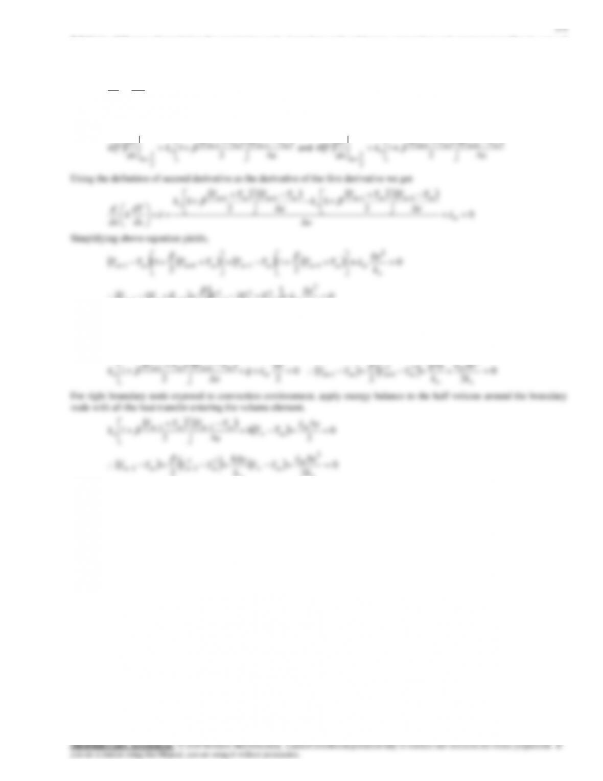
5-4C The energy balance method is based on subdividing the medium into a sufficient number of volume elements, and then
5-5C The analytical solutions are based on (1) driving the governing differential equation by performing an energy balance
on a differential volume element, (2) expressing the boundary conditions in the proper mathematical form, and (3) solving the
5-3
Finite Difference Formulation of Differential Equations
5-7C A point at which the finite difference formulation of a problem is obtained is called a node, and all the nodes for a
5-8 The finite difference formulation of steady two–dimensional heat conduction in a medium with heat generation and
constant thermal conductivity is given by
22 ,
1,,1,
,1,,1 =+
+−
+− +−+−
e
TTT
TTT nmnmnmnmnmnmnm
5-5
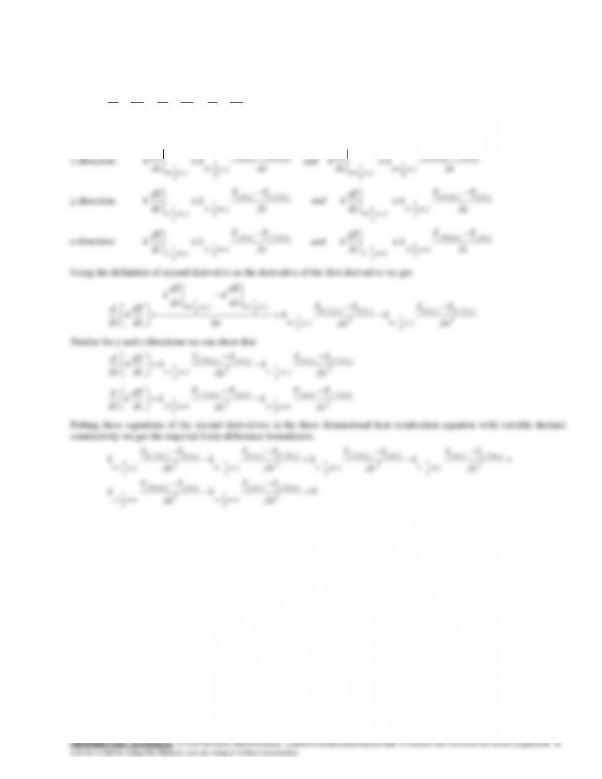
5-10 For a three dimensional steady state heat transfer without internal heat generation finite difference formulations are to be
determined.
Analysis The three dimensional heat conduction equation for steady state conditions with variable thermal conductivity is
expressed as
0=
+
+
z
T
k
zy
T
k
yx
T
k
x
Using Eq. (5-6), the first derivative of the temperature at the midpoints surrounding the node can be expressed for x, y and z
directions as
TT
dT
TT
dT
jnmjnm
,,,,1
,,1,,
−
−
−
5-7
One-Dimensional Steady Heat Conduction
5-13C The finite difference form of a heat conduction problem by the energy balance method is obtained by subdividing the
medium into a sufficient number of volume elements, and then applying an energy balance on each element. This is done by
5-14C The basic steps involved in the iterative Gauss-Seidel method are: (1) Writing the equations explicitly for each
5-15C In a medium in which the finite difference formulation of a general interior node is given in its simplest form as
2
11 =+
+− +−
e
TTT mmmm
5-8
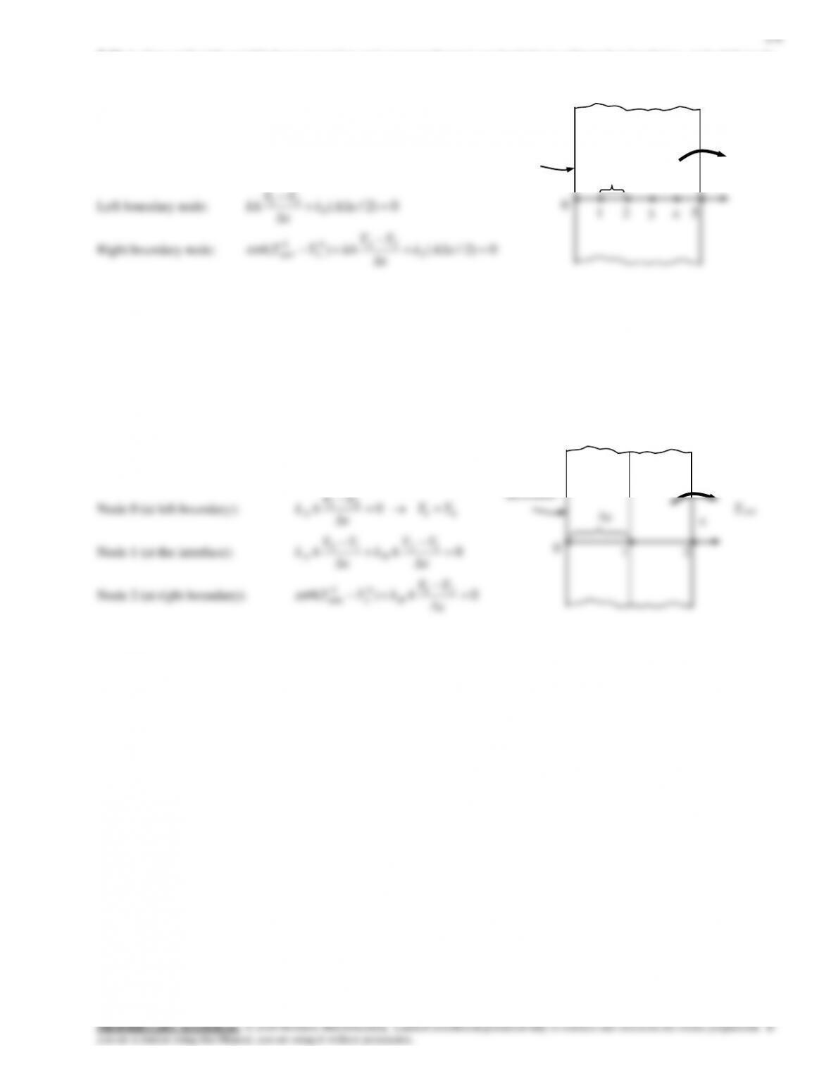
5-19 A plane wall with no heat generation is subjected to specified temperature at the left (node 0) and heat flux at the right
boundary (node 8). The finite difference formulation of the boundary nodes and the finite difference formulation for the rate
of heat transfer at the left boundary are to be determined.
Assumptions 1 Heat transfer through the wall is given to be steady, and the thermal conductivity to be constant. 2 Heat
transfer is one-dimensional since the plate is large relative to its thickness. 3 There is no heat generation in the medium.
Analysis Using the energy balance approach and taking the direction of all heat
transfers to be towards the node under consideration, the finite difference
formulations become
•
•
•
•
•
•
•
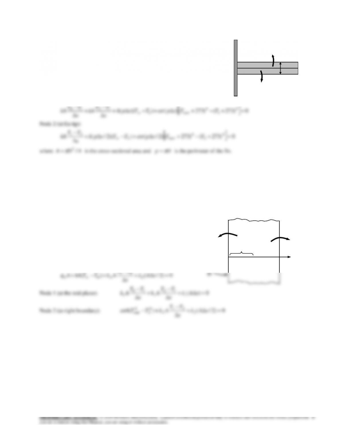
5-20 A plane wall with variable heat generation and constant thermal conductivity is subjected to uniform heat flux
0
q
at the
left (node 0) and convection at the right boundary (node 4). The finite difference formulation of the boundary nodes is to be
determined.
Assumptions 1 Heat transfer through the wall is given to be steady, and the
thermal conductivity to be constant. 2 Heat transfer is one-dimensional since
the plate is large relative to its thickness. 3 Radiation heat transfer is negligible.
Analysis Using the energy balance approach and taking the direction of all heat
transfers to be towards the node under consideration, the finite difference
formulations become
01
−
TT
x
)(xe
1
h, T
•
•
•
•
•
0
2
3
4
0
q
5-10
5-23 A pin fin with negligible heat transfer from its tip is considered. The complete finite difference formulation for the
determination of nodal temperatures is to be obtained.
Assumptions 1 Heat transfer through the pin fin is given to be steady and one–
dimensional, and the thermal conductivity to be constant. 2 Convection heat
transfer coefficient is constant and uniform. 3 Heat loss from the fin tip is given
to be negligible.
Analysis The nodal network consists of 3 nodes, and the base temperature T0 at
node 0 is specified. Therefore, there are two unknowns T1 and T2, and we need
two equations to determine them. Using the energy balance approach and taking
the direction of all heat transfers to be towards the node under consideration, the
finite difference formulations become
Node 1 (at midpoint):
0)273()273()())((4
1
4
surr1
12
10 =+−++−+
−
+
−
TTxpTTxph
x
TT
kA
x
TT
kA
Node 2 (at fin tip):
0)273()273()2/())(2/( 4
2
4
surr2
21 =+−++−+
−
TTxpTTxph
x
TT
kA
where
4/
2
DA
=
is the cross-sectional area and
Dp
=
is the perimeter of the fin.
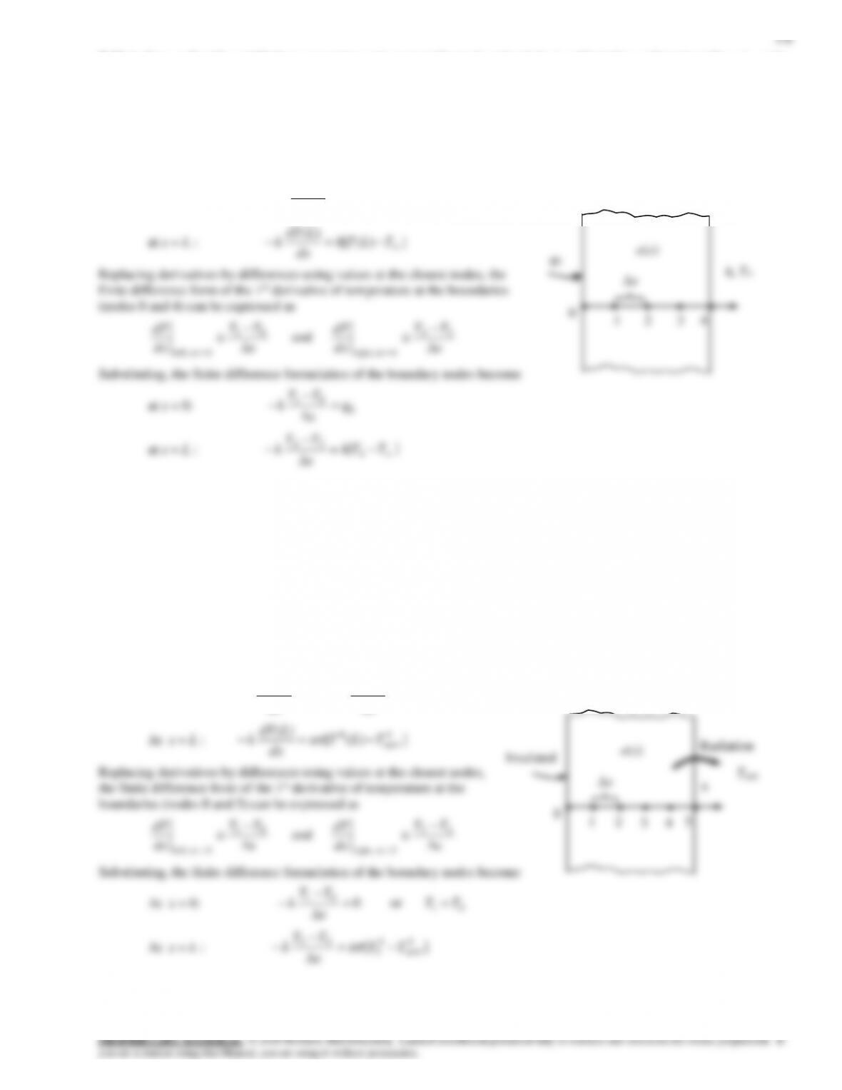
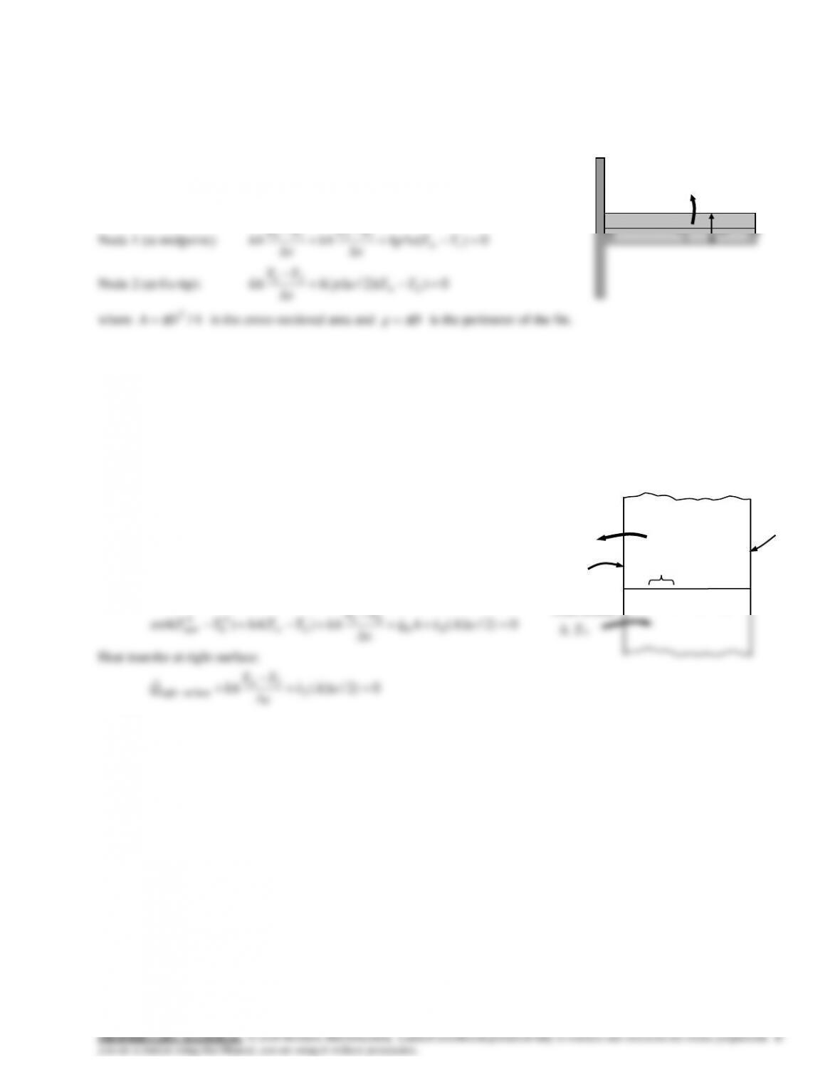
5-24 A plane wall with variable heat generation and variable thermal conductivity is subjected to specified heat flux
0
q
and
convection at the left boundary (node 0) and radiation at the right boundary (node 5). The complete finite difference
formulation of this problem is to be obtained.
Assumptions 1 Heat transfer through the wall is given to be steady
and one-dimensional, and the thermal conductivity and heat
generation to be variable. 2 Convection heat transfer at the right
surface is negligible.
Analysis Using the energy balance approach and taking the
direction of all heat transfers to be towards the node under
consideration, the finite difference formulations become
Node 0 (at left boundary):
01
−
TT
x
Convectio
T0
h, T
•
•
•
0
1
2
D
x
Tsurr
Radiation
Convectio
x
1
•
•
•
0
2
q0
Tsurr
Radiation
h, T
k(T)
)(xe
5-11
5-25 A pin fin with negligible heat transfer from its tip is considered. The complete finite difference formulation for the
determination of nodal temperatures is to be obtained.
Assumptions 1 Heat transfer through the pin fin is given to be steady and one-dimensional, and the thermal conductivity to
be constant. 2 Convection heat transfer coefficient is constant and uniform. 3 Radiation heat transfer is negligible. 4 Heat
loss from the fin tip is given to be negligible.
Analysis The nodal network consists of 3 nodes, and the base temperature T0 at
node 0 is specified. Therefore, there are two unknowns T1 and T2, and we need
two equations to determine them. Using the energy balance approach and taking
the direction of all heat transfers to be towards the node under consideration, the
finite difference formulations become
12
10 =−+
−
−
TT
TT
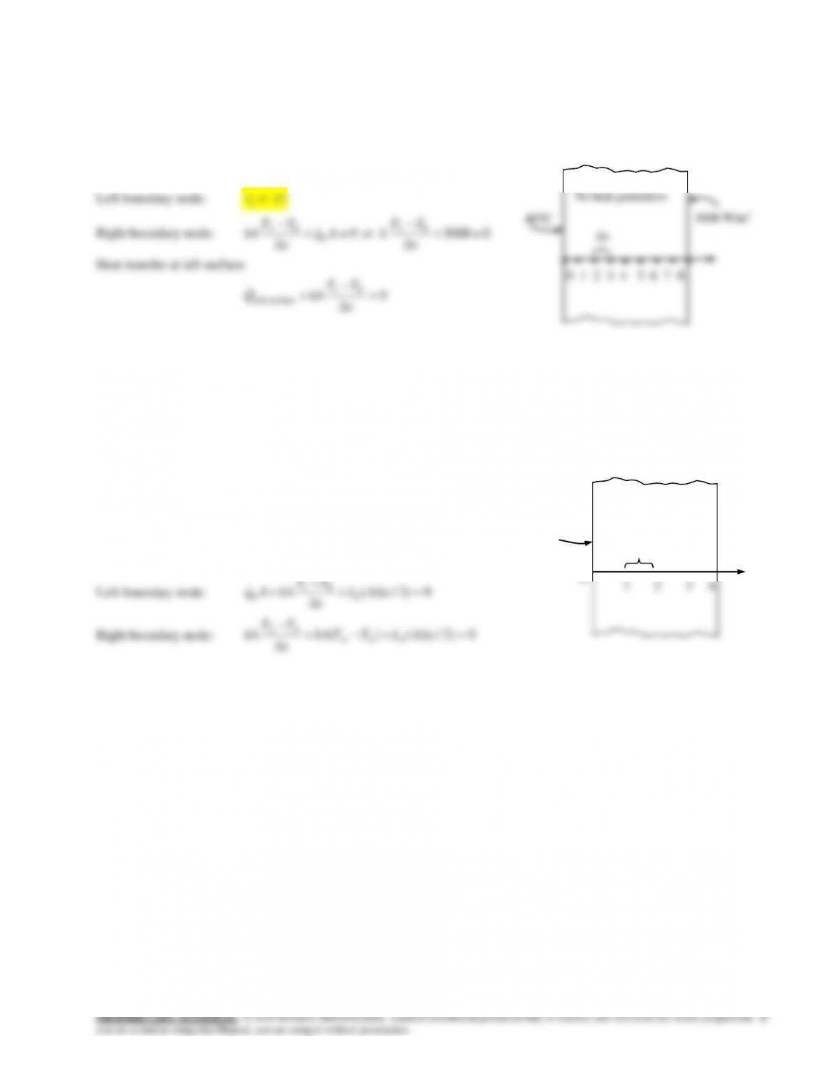
5-26 A plane wall with variable heat generation and constant thermal conductivity is subjected to combined convection,
radiation, and heat flux at the left (node 0) and specified temperature at the right boundary (node 5). The finite difference
formulation of the left boundary node (node 0) and the finite difference formulation for the rate of heat transfer at the right
boundary (node 5) are to be determined.
Assumptions 1 Heat transfer through the wall is given to be
steady and one-dimensional. 2 The thermal conductivity is
given to be constant.
Analysis Using the energy balance approach and taking the
direction of all heat transfers to be towards the node under
consideration, the finite difference formulations become
Left boundary node (all temperatures are in K):
0)2/()()( 00
01
0
4
0
4
surr =++
−
+−+− xAeAq
x
TT
kATThATTA
Heat transfer at right surface:
0)2/(
5
54
surfaceright =+
−
+xAe
x
TT
kAQ
Convectio
T0
h, T
•
•
•
0
1
2
D
x
Convection
x
e(x)
1
•
•
•
•
•
0
2
3
4
•
5
Tsurr
Radiation
q0
h, T
Ts
5-13
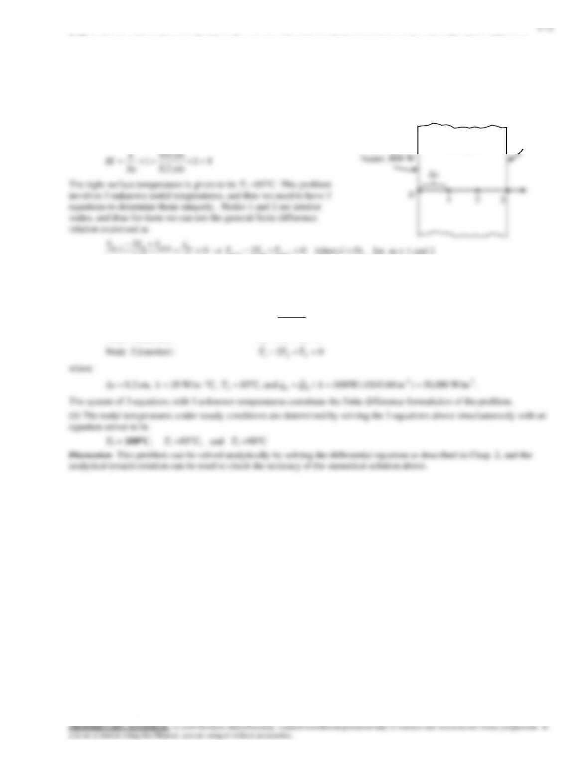
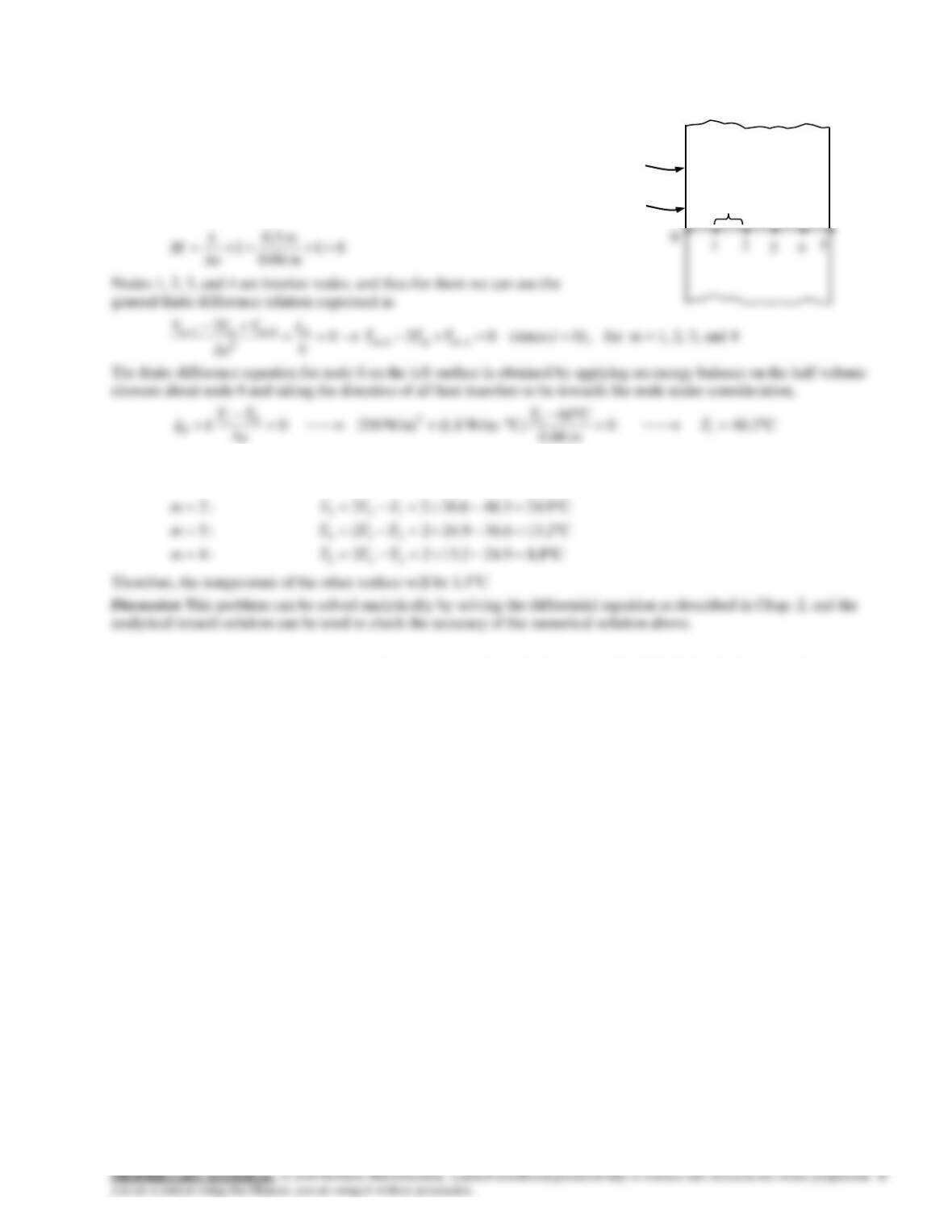
5-28 A plane wall is subjected to specified heat flux and specified temperature on one side, and no conditions on the other.
The finite difference formulation of this problem is to be obtained, and the temperature of the other side under steady
conditions is to be determined.
Assumptions 1 Heat transfer through the plate is given to be steady and one–
dimensional. 2 There is no heat generation in the plate.
PropertiesThe thermal conductivity is given to be k = 1.8 W/m°C.
Analysis The nodal spacing is given to be x=0.06 m.
Then the number of nodes M becomes
3
m 3.0
L
m 0.06
x
Other nodal temperatures are determined from the general interior node relation as follows:
=−=−==
=−=−==
C9.243.486.3622 :2
C6.36603.4822 :1
123
012
TTTm
TTTm
x
•
•
•
•
•
0
•
T0
0
q
5-14
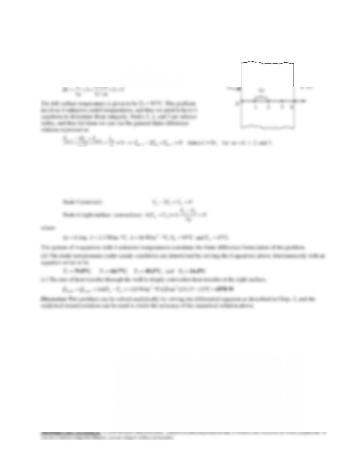
5-29 A plane wall is subjected to specified temperature on one side and convection on the other. The finite difference
formulation of this problem is to be obtained, and the nodal temperatures under steady conditions as well as the rate of heat
transfer through the wall are to be determined.
Assumptions 1 Heat transfer through the wall is given to be steady and one-dimensional. 2 Thermal conductivity is constant.
3 There is no heat generation. 4 Radiation heat transfer is negligible.
Properties The thermal conductivity is given to be k = 2.3 W/m°C.
Analysis The nodal spacing is given to be x=0.1 m. Then the
number of nodes M becomes
m 4.0
L
T0
h, T
e
5-15
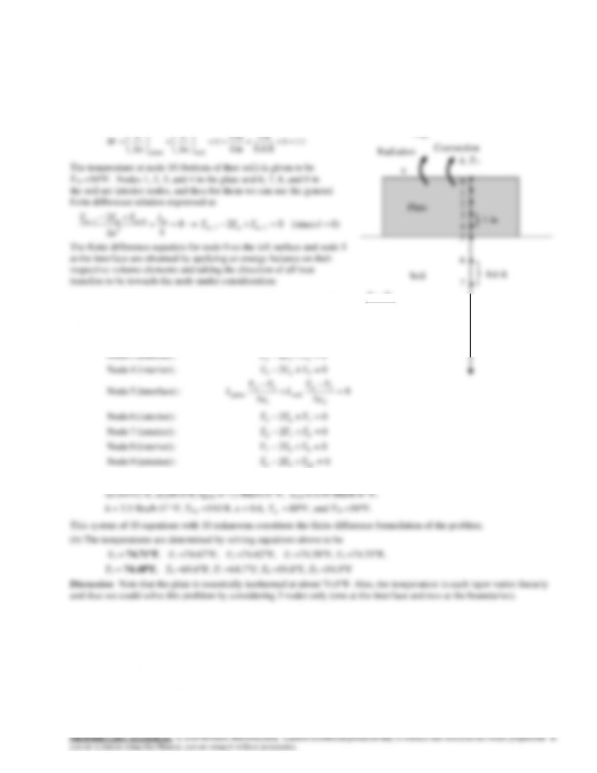
5-30E A large plate lying on the ground is subjected to convection and radiation. Finite difference formulation is to be
obtained, and the top and bottom surface temperatures under steady conditions are to be determined.
Assumptions 1 Heat transfer through the plate is given to be steady and one-dimensional. 2 There is no heat generation in
the plate and the soil. 3 Thermal contact resistance at plate-soil interface is negligible.
Properties The thermal conductivity of the plate and the soil are given to be kplate = 7.2 Btu/hft°F and ksoil = 0.49 Btu/hft°F.
Analysis The nodal spacing is given to be x1=1 in. in the plate, and be x2=0.6 ft in the soil. Then the number of nodes
becomes
111
ft 0.6
ft 3
in 1
in 5
1
soilplate
=++=+
+
=x
L
x
L
M
The temperature at node 10 (bottom of thee soil) is given to be
T10 =50F. Nodes 1, 2, 3, and 4 in the plate and 6, 7, 8, and 9 in
the soil are interior nodes, and thus for them we can use the general
finite difference relation expressed as
)0 (since 02 0
2
11
2
11 ==+−→=+
+−
+−
+− eTTT
k
e
x
TTT
mmm
mmmm
The finite difference equation for node 0 on the left surface and node 5
at the interface are obtained by applying an energy balance on their
respective volume elements and taking the direction of all heat
transfers to be towards the node under consideration:
0 :)(interface 5 Node
02 :(interior) 4 Node
02 :(interior) 3 Node
02 :(interior) 2 Node
02 :(interior) 1 Node
0])460([)( :surface) (top 0 Node
2
56
soil
1
54
plate
543
432
321
210
1
01
plate
4
0
4
0
=
−
+
−
=+−
=+−
=+−
=+−
=
−
++−+−
x
TT
k
x
TT
k
TTT
TTT
TTT
TTT
x
TT
kTTTTh sky
02 :(interior) 9 Node
02 :(interior) 8 Node
02 :(interior) 7 Node
02 :(interior) 6 Node
1098
987
876
765
=+−
=+−
=+−
=+−
TTT
TTT
TTT
TTT
where
Convection
h, T
0.6 ft
Soil
Tsky
Radiation
•
•
•
•
•
•
•
•
•
•
•
0
1
2
3
4
5
6
7
8
9
10
1 in
Plate
5-17
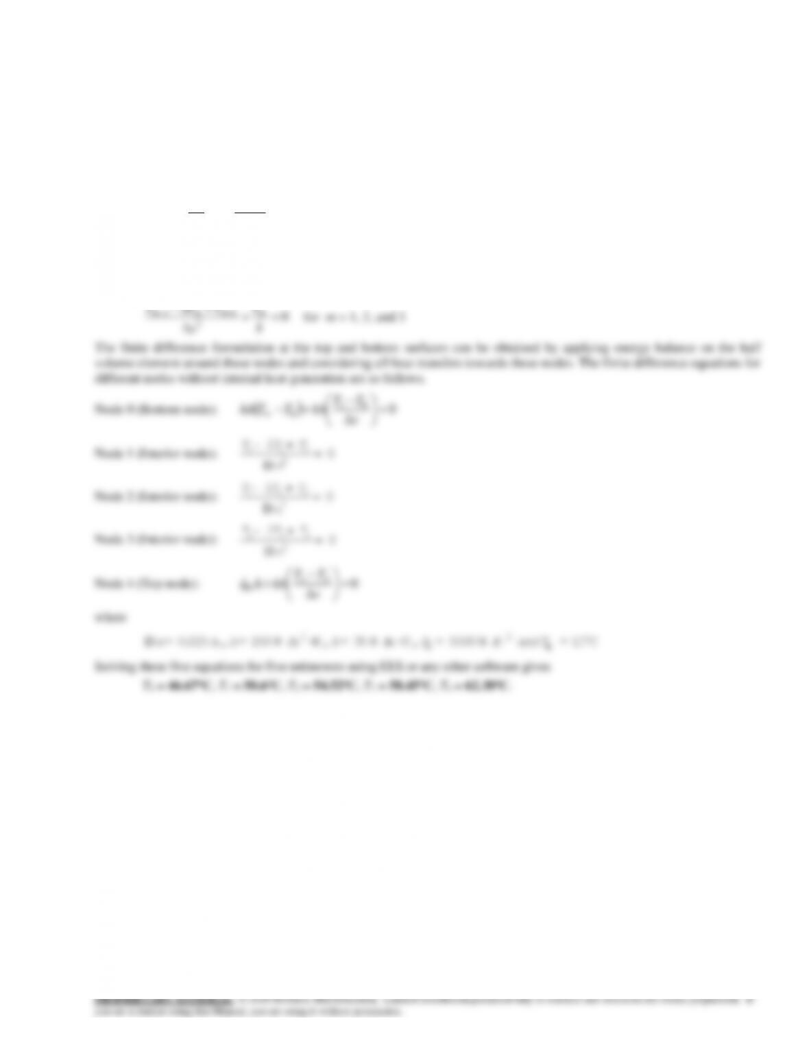
5-32 A steel plate with no internal heat generation is subjected to a uniform heat flux on its top surface while the bottom
surface is cooled convectively by a fluid at 10oC and having h = 150 W/m2·K. Using finite difference formulation, the
temperature at the midpoint of the plate is to be determined.
Assumptions 1 Steady state 1-D heat transfer in lateral direction. 2 Constant thermal conductivity of the steel plate.
Properties Thermal conductivity of the steel plate is given as 35 W/m·K.
Analysis To discretize the plate of thickness 0.1 m into four equal parts, each part must be of length 0.025 m i.e.,
0.025 mx=
And hence the number of nodes is
5
025.0
1.0
11 =+=
+= x
L
M
This problem involves 5 unknown nodal temperatures and hence we need 5 equations to determine these temperatures. The
steel plate thickness is discretized such that the node 0 is on the bottom of the plate exposed to convective environment while
the node 4 is on the top surface exposed to the uniform heat flux. Nodes 1, 2 and 3 are the internal nodes and their
temperature can be expressed using general form of the finite difference formulation.
0
2
2
11 =+
+− +−
k
e
x
TTT mmmm
for m = 1, 2, and 3
The finite difference formulation at the top and bottom surfaces can be obtained by applying energy balance on the half
volume element around these nodes and considering all heat transfers towards these nodes. The finite difference equations for
different nodes without internal heat generation are as follows.
Node 0 (Bottom node):
( )
0
01
0=
−
+−
x
TT
kATThA
Node 1 (Interior node):
0 1 2
2
20
T T T
x
-+
=
D
Node 2 (Interior node):
1 2 3
2
20
T T T
x
-+
=
D
Node 3 (Interior node):
2 3 4
2
20
T T T
x
-+
=
D
Node 4 (Top node):
0
43
0=
−
+x
TT
kAAq
where
22
0
0.025 m , 150 W /m K , 35 W /m K , 5500 W /m 10 Cx h k q and T
¥
D = = × = × = = °
Solving these five equations for five unknowns using EES or any other software gives
T0 = 46.67oC, T1 = 50.6oC, T2 = 54.52oC, T3 = 58.45oC, T4 = 62.38oC.
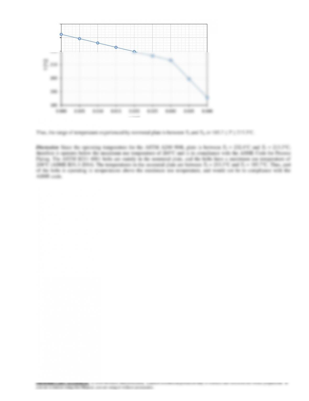
5-19
180
190
200
210
220
230
240
0.000 0.005 0.010 0.015 0.020 0.025 0.030 0.035 0.040
T [°C]
x [m]
5-20
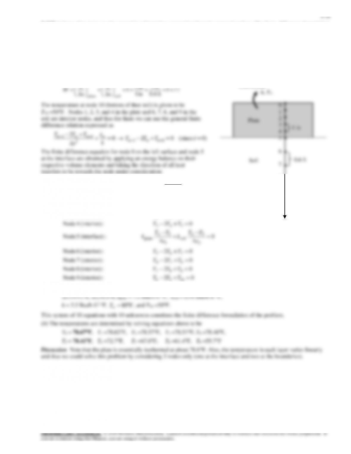
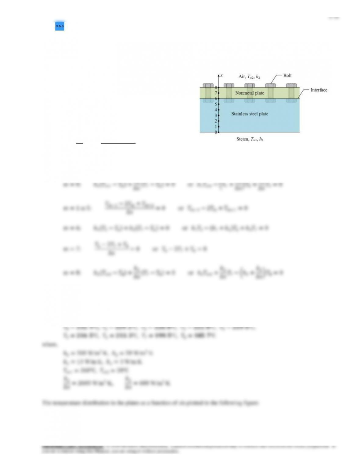
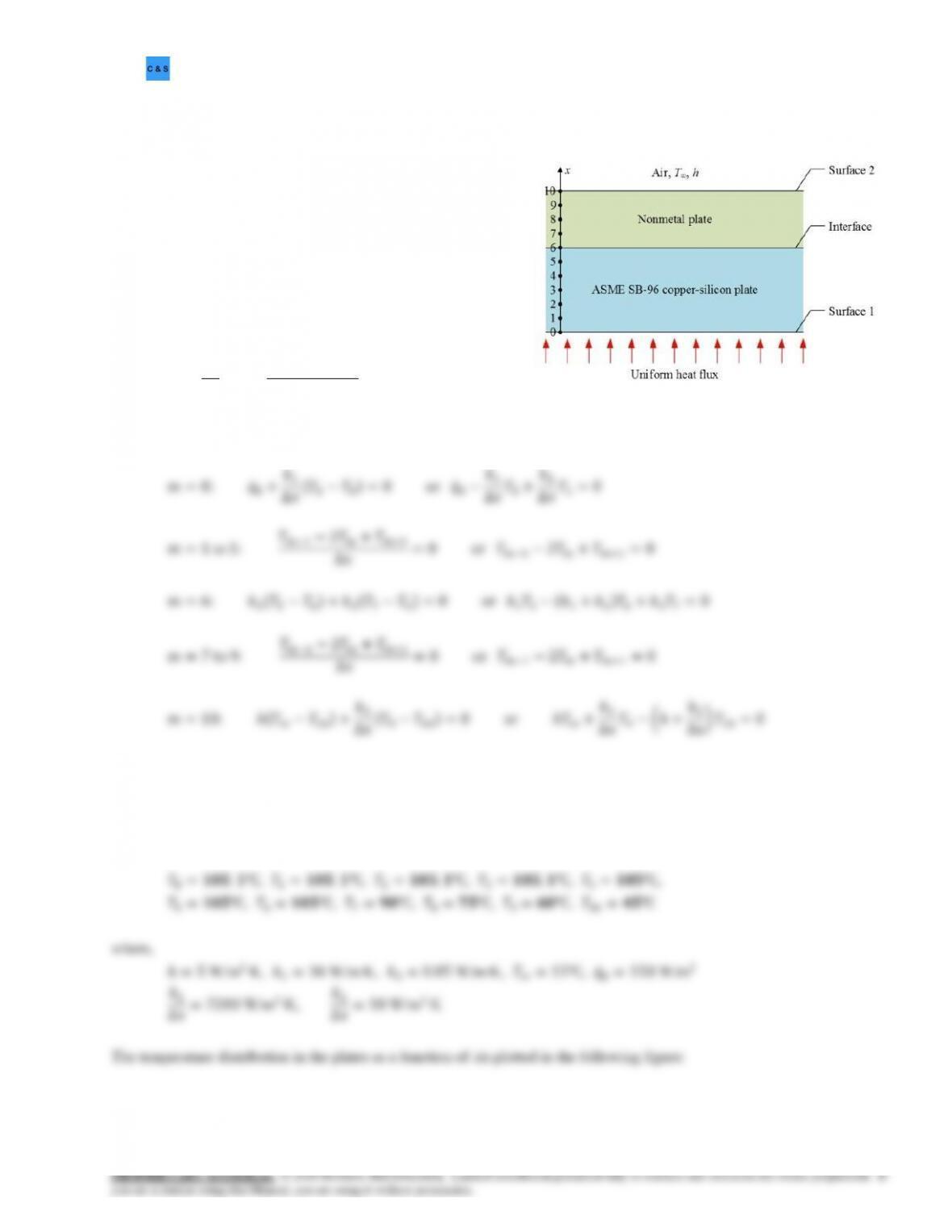
5-34 A nonmetal plate and an ASME SB-96 copper-silicon plate are attached together. The bottom surface is subjected
to uniform heat flux. The top surface is exposed to convection heat transfer. Determine the nodal temperatures, and whether
the use of the ASME SB-96 plate complies with the ASME Boiler and Pressure Vessel Code. Also, what is the lowest value
of the convection heat transfer coefficient for the air on the upper surface so that the ASME SB-96 plate is below 93°C?
Assumptions1 Heat transfer is steady. 2 One dimensional heat
conduction through plates. 3 Uniform heat flux on bottom
surface. 4 Uniform surface temperature. 5 No contact resistance
at the interface. 6 Thermal properties are constant. 7 Thermal
radiation is negligible.
Properties The thermal conductivity for the ASME SB–96
copper-silicon plate is given as k1 = 36 W/m·K, and for the
nonmetal plate as k2 = 0.05 W/m·K.
Analysis The nodal spacing is given as Δx = 5 mm. So, the
number of nodes is
𝑀 = 𝐿
∆𝑥 +1 = (30+20)mm
5 mm +1 = 11
The nodes are numbered from m = 0 to 10. The finite difference formulations for the nodes are
Note that node 0 is a specified heat flux boundary; nodes 1–5 and 7–9 are interior nodes; node 6 is an interface boundary;
node 10 is a convection boundary.
Solving for the nodal temperatures, T0 to T10, yields
𝑇0=𝟏𝟎𝟓.𝟏℃, 𝑇1=𝟏𝟎𝟓.𝟏℃, 𝑇2=𝟏𝟎𝟓.𝟏℃, 𝑇3=𝟏𝟎𝟓.𝟏℃, 𝑇4=𝟏𝟎𝟓℃,