B-202 SOLUTIONS
Solutions to Questions and Problems
NOTE: All end of chapter problems were solved using a spreadsheet. Many problems require multiple steps.
Due to space and readability constraints, when these intermediate steps are included in this solutions
manual, rounding may appear to have occurred. However, the final answer for each problem is found
without rounding during any step in the problem.
Basic
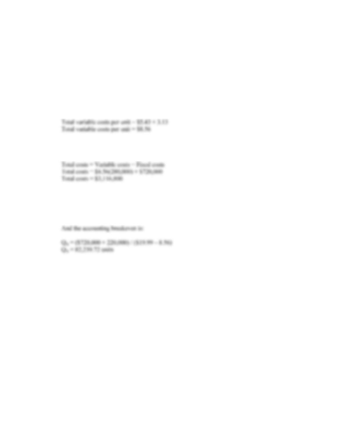
1. a. The total variable cost per unit is the sum of the two variable costs, so:
b. The total costs include all variable costs and fixed costs. We need to make sure we are including
all variable costs for the number of units produced, so:
c. The cash breakeven, that is the point where cash flow is zero, is:
Q C = $720,000 / ($19.99 – 8.56)
Q C = 62,992.13 units
2. The total costs include all variable costs and fixed costs. We need to make sure we are including all
variable costs for the number of units produced, so:
Total costs = ($24.86 + 14.08)(120,000) + $1,550,000
Total costs = $6,222,800
The marginal cost, or cost of producing one more unit, is the total variable cost per unit, so:
Marginal cost = $24.86 + 14.08
Marginal cost = $38.94
CHAPTER 11 B-203
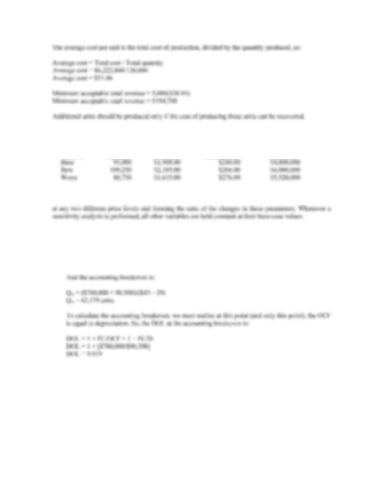
3. The base-case, best-case, and worst-case values are shown below. Remember that in the best-case, sales
and price increase, while costs decrease. In the worst-case, sales and price decrease, and costs increase.
Unit
Scenario Unit Sales Unit Price Variable Cost Fixed Costs
4. An estimate for the impact of changes in price on the profitability of the project can be found from the
sensitivity of NPV with respect to price: NPV/P. This measure can be calculated by finding the NPV
5. a. To calculate the accounting breakeven, we first need to find the depreciation for each year. The
depreciation is:
Depreciation = $724,000/8
Depreciation = $90,500 per year
b. We will use the tax shield approach to calculate the OCF. The OCF is:
OCFbase = [(P – v)Q – FC](1 – tc) + tcD
OCFbase = [($43 – 29)(90,000) – $780,000](0.65) + 0.35($90,500)
OCFbase = $343,675
B-204 SOLUTIONS
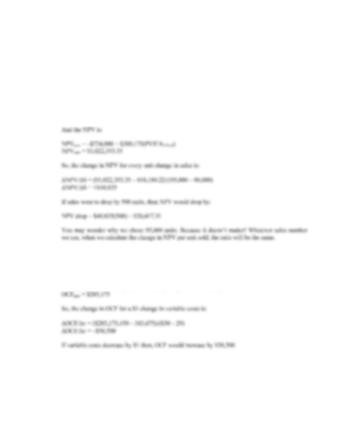
Now we can calculate the NPV using our base-case projections. There is no salvage value or
NWC, so the NPV is:
NPVbase = –$724,000 + $343,675(PVIFA15%,8)
NPVbase = $818,180.22
To calculate the sensitivity of the NPV to changes in the quantity sold, we will calculate the NPV
at a different quantity. We will use sales of 95,000 units. The NPV at this sales level is:
OCFnew = [($43 – 29)(95,000) – $780,000](0.65) + 0.35($90,500)
OCFnew = $389,175
c. To find out how sensitive OCF is to a change in variable costs, we will compute the OCF at a
variable cost of $30. Again, the number we choose to use here is irrelevant: We will get the same
ratio of OCF to a one dollar change in variable cost no matter what variable cost we use. So, using
the tax shield approach, the OCF at a variable cost of $30 is:
OCFnew = [($43 – 30)(90,000) – 780,000](0.65) + 0.35($90,500)
CHAPTER 11 B-205
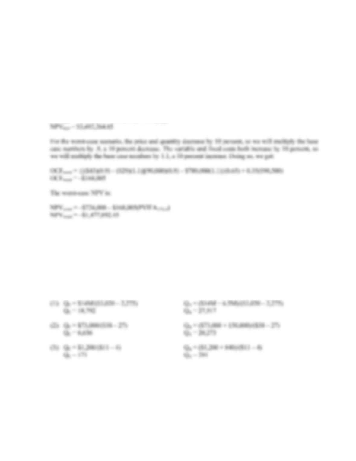
6. We will use the tax shield approach to calculate the OCF for the best- and worst-case scenarios. For the
best-case scenario, the price and quantity increase by 10 percent, so we will multiply the base case
numbers by 1.1, a 10 percent increase. The variable and fixed costs both decrease by 10 percent, so we
will multiply the base case numbers by .9, a 10 percent decrease. Doing so, we get:
OCFbest = {[($43)(1.1) – ($29)(0.9)](90,000)(1.1) – $780,000(0.9)}(0.65) + 0.35($90,500)
OCFbest = $939,595
The best-case NPV is:
NPVbest = –$724,000 + $939,595(PVIFA15%,8)
7. The cash breakeven equation is:
Q
C = FC/(P – v)
And the accounting breakeven equation is:
Q
A = (FC + D)/(P – v)
Using these equations, we find the following cash and accounting breakeven points:
B-206 SOLUTIONS
8. We can use the accounting breakeven equation:
Q
A = (FC + D)/(P – v)
to solve for the unknown variable in each case. Doing so, we find:
9. The accounting breakeven for the project is:
Q
A = [$6,000 + ($18,000/4)]/($57 – 32)
Q
A = 540
And the cash breakeven is:
Q
C = $9,000/($57 – 32)
Q
C = 360
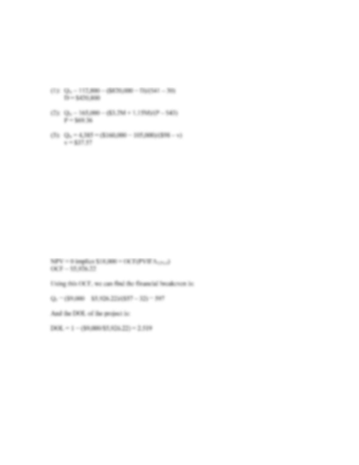
At the financial breakeven, the project will have a zero NPV. Since this is true, the initial cost of the
project must be equal to the PV of the cash flows of the project. Using this relationship, we can find the
OCF of the project must be:
10. In order to calculate the financial breakeven, we need the OCF of the project. We can use the cash and
accounting breakeven points to find this. First, we will use the cash breakeven to find the price of the
product as follows:
Q
C = FC/(P – v)
13,200 = $140,000/(P – $24)
P = $34.61
CHAPTER 11 B-207
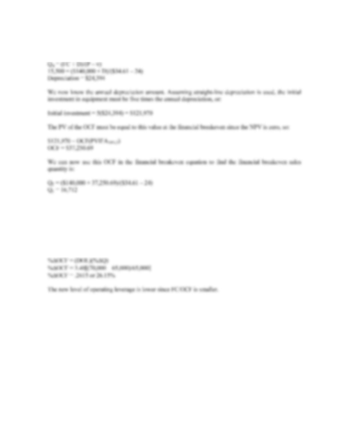
Now that we know the product price, we can use the accounting breakeven equation to find the
depreciation. Doing so, we find the annual depreciation must be:
11. We know that the DOL is the percentage change in OCF divided by the percentage change in quantity
sold. Since we have the original and new quantity sold, we can use the DOL equation to find the
percentage change in OCF. Doing so, we find:
DOL = %OCF / %Q
Solving for the percentage change in OCF, we get:
12. Using the DOL equation, we find:
DOL = 1 + FC / OCF
3.40 = 1 + $130,000/OCF
OCF = $54,167
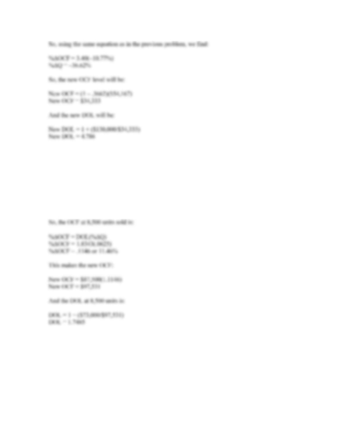
The percentage change in quantity sold at 58,000 units is:
%ΔQ = (58,000 – 65,000) / 65,000
%ΔQ = –.1077 or –10.77%
B-208 SOLUTIONS
13. The DOL of the project is:
DOL = 1 + ($73,000/$87,500)
DOL = 1.8343
If the quantity sold changes to 8,500 units, the percentage change in quantity sold is:
%Q = (8,500 – 8,000)/8,000
%ΔQ = .0625 or 6.25%
14. We can use the equation for DOL to calculate fixed costs. The fixed cost must be:
DOL = 2.35 = 1 + FC/OCF
FC = (2.35 – 1)$41,000
FC = $58,080
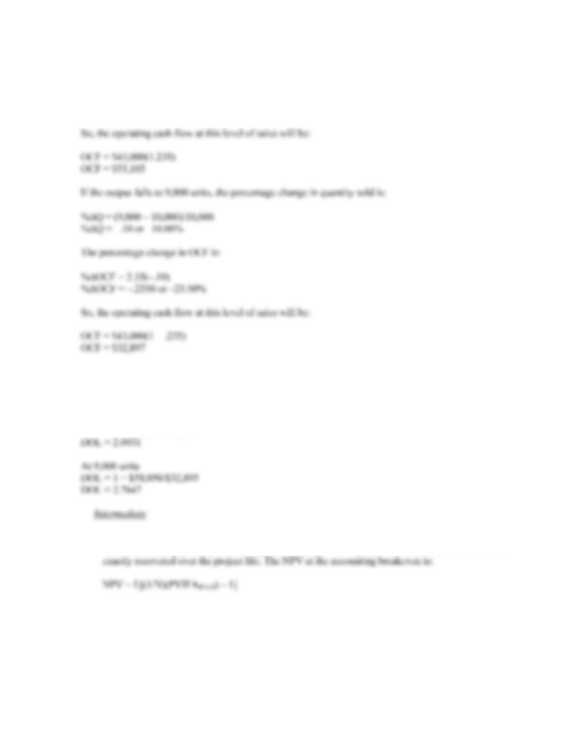
If the output rises to 11,000 units, the percentage change in quantity sold is:
%Q = (11,000 – 10,000)/10,000
%ΔQ = .10 or 10.00%
CHAPTER 11 B-209
The percentage change in OCF is:
%OCF = 2.35(.10)
%ΔOCF = .2350 or 23.50%
15. Using the equation for DOL, we get:
DOL = 1 + FC/OCF
At 11,000 units
DOL = 1 + $58,050/$53,105
16. a. At the accounting breakeven, the IRR is zero percent since the project recovers the initial
investment. The payback period is N years, the length of the project since the initial investment is
b. At the cash breakeven level, the IRR is –100 percent, the payback period is negative, and the NPV
is negative and equal to the initial cash outlay.
B-210 SOLUTIONS
c. The definition of the financial breakeven is where the NPV of the project is zero. If this is true,
then the IRR of the project is equal to the required return. It is impossible to state the payback
17. Using the tax shield approach, the OCF at 110,000 units will be:
OCF = [(P – v)Q – FC](1 – tC) + tC(D)
OCF = [($32 – 19)(110,000) – 210,000](0.66) + 0.34($490,000/4)
OCF = $846,850
We will calculate the OCF at 111,000 units. The choice of the second level of quantity sold is arbitrary
and irrelevant. No matter what level of units sold we choose, we will still get the same sensitivity. So,
the OCF at this level of sales is:
18. At 110,000 units, the DOL is:
DOL = 1 + FC/OCF
DOL = 1 + ($210,000/$846,850)
DOL = 1.2480