ΑBC “
!1#!L
R“2“Cos#Θ$
!! L
R“2#Cos#Θ$2“3%2
ΩAB
2;
Parameters “&ΩAB &5700.
2Π
60.0
,R&
48.5
1000.
,L&
141.0
1000.
,d&
36.4
1000.
,mD&0.439, (D&0.00144, mC&0.434‘;
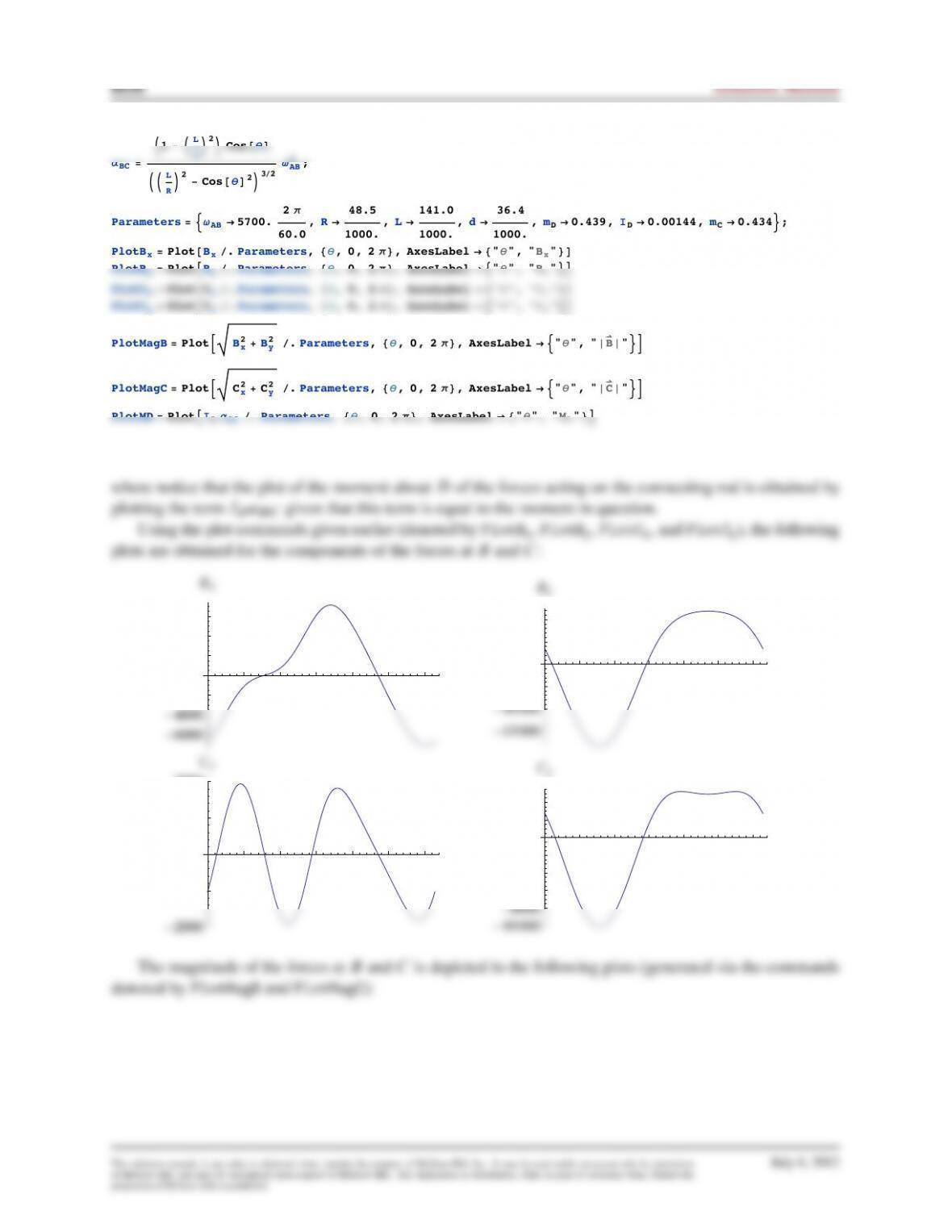
PlotBx“Plot#Bx%.Parameters,(Θ, 0, 2 Π), AxesLabel &(“Θ“, “Bx“)$
PlotBy“Plot*By%.Parameters,(Θ, 0, 2 Π), AxesLabel &+“Θ“, “By“,–
PlotCx“Plot#Cx%.Parameters,(Θ, 0, 2 Π), AxesLabel &(“Θ“, “Cx“)$
PlotCy“Plot*Cy%.Parameters,(Θ, 0, 2 Π), AxesLabel &+“Θ“, “Cy“,–
PlotMagB “Plot.Bx
2)By
2%.Parameters,(Θ, 0, 2 Π), AxesLabel &&“Θ“, “/B
0/“‘1
PlotMagC “Plot.Cx
2)Cy
2%.Parameters,(Θ, 0, 2 Π), AxesLabel &&“Θ“, “/C
0/“‘1
PlotMD “Plot*(DΑBC %.Parameters,(Θ, 0, 2 Π), AxesLabel &(“Θ“, “MD“)–
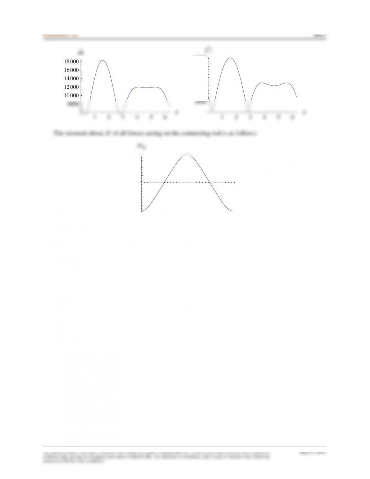
where notice that the plot of the moment about
D
of the forces acting on the connecting rod is obtained by
plotting the term ID˛BC given that this term is equal to the moment in question.
Using the plot commands given earlier (denoted by
PlotBx
,
PlotBy
,
PlotCx
, and
PlotCy
), the following
plots are obtained for the components of the forces at Band C:
1
2
3
4
5
6
Θ
“6000
“4000
“2000
2000
4000
6000
Bx
1
2
3
4
5
6
Θ
“15 000
“10 000
“5000
5000
10 000
By
1
2
3
4
5
6
Θ
“1000
1000
2000
Cx
1
2
3
4
5
6
Θ
“8000
“6000
“4000
“2000
2000
4000
Cy
The magnitude of the forces at
B
and
C
is depicted in the following plots (generated via the commands
denoted by PlotMagB and PlotMagC):
This solutions manual, in any print or electronic form, remains the property of McGraw-Hill, Inc. It may be used and/or possessed only by permission
of McGraw-Hill, and must be surrendered upon request of McGraw-Hill. Any duplication or distribution, either in print or electronic form, without the
permission of McGraw-Hill, is prohibited.
July 6, 2012
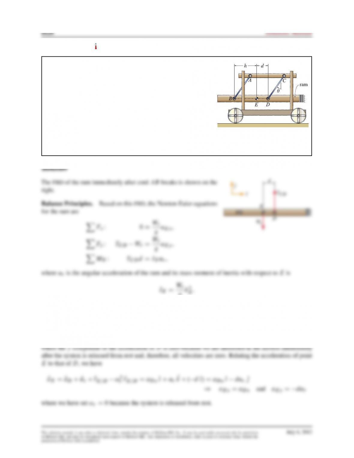
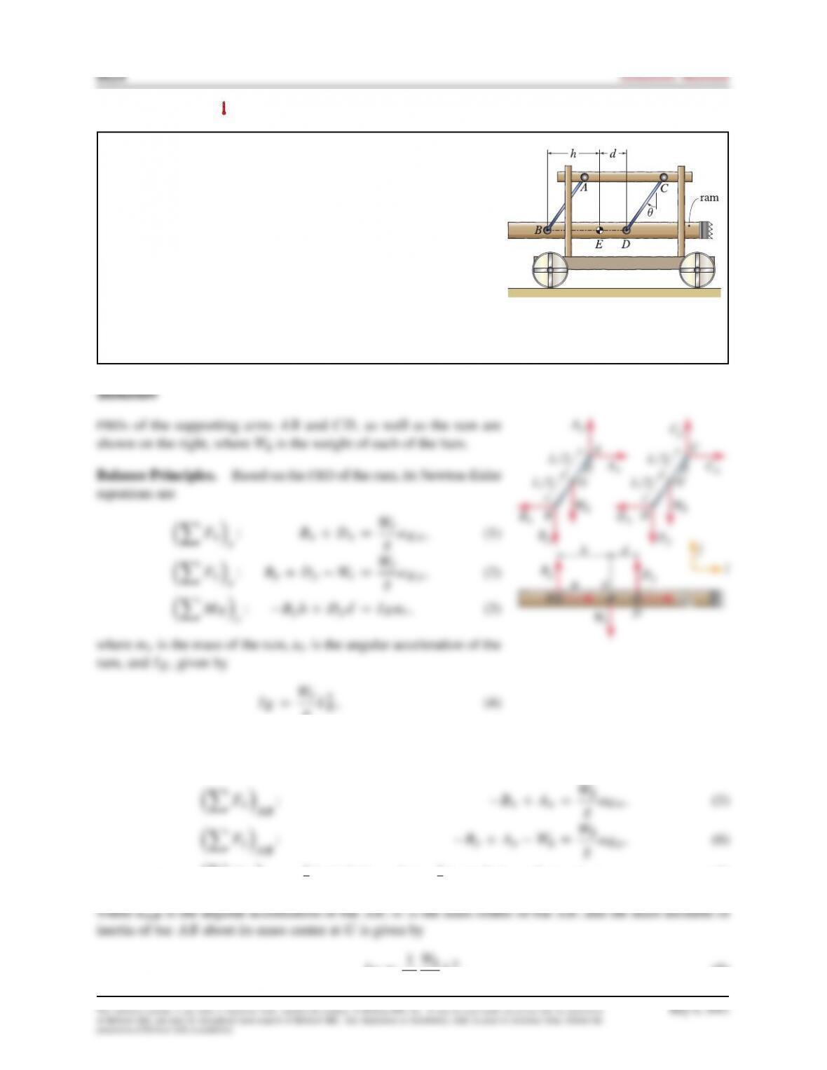
Problem 7.101
The figure shows a weapon called a battering ram (modern large
battering rams are typically mounted on armored vehicles). The
ram has a weight
WrD2500 lb
, center of mass at
E
, and radius of
gyration
kED6:5 ft
. Also let the distance between points
A
and
B
and between points
C
and
D
be
6ft
. In addition, let
hD4:5 ft
and
dD3ft
. Finally, let the connections at points
A
,
B
,
C
, and
D
be
pin connections, and assume that the cart does not move while the
ram swings.
Assuming that the ram is suspended by inextensible cords of
negligible mass, determine the tension in the cords and the accel-
eration of
E
immediately after the ram is released from rest at
D75ı.
gk2
Force Laws. All forces have been accounted for on the FBD.
Kinematic Equations.
Because we are interested in what is happening immediately after the ram is
released from rest, all velocities are zero. Because of this and because the motion of the ram is a curvilinear
translation, the acceleration of every point on the ram must be perpendicular to the segments
AB
and
CD
.
of McGraw-Hill, and must be surrendered upon request of McGraw-Hill. Any duplication or distribution, either in print or electronic form, without the
permission of McGraw-Hill, is prohibited.
Dynamics 2e 1619
the solution of which is
of McGraw-Hill, and must be surrendered upon request of McGraw-Hill. Any duplication or distribution, either in print or electronic form, without the
permission of McGraw-Hill, is prohibited.
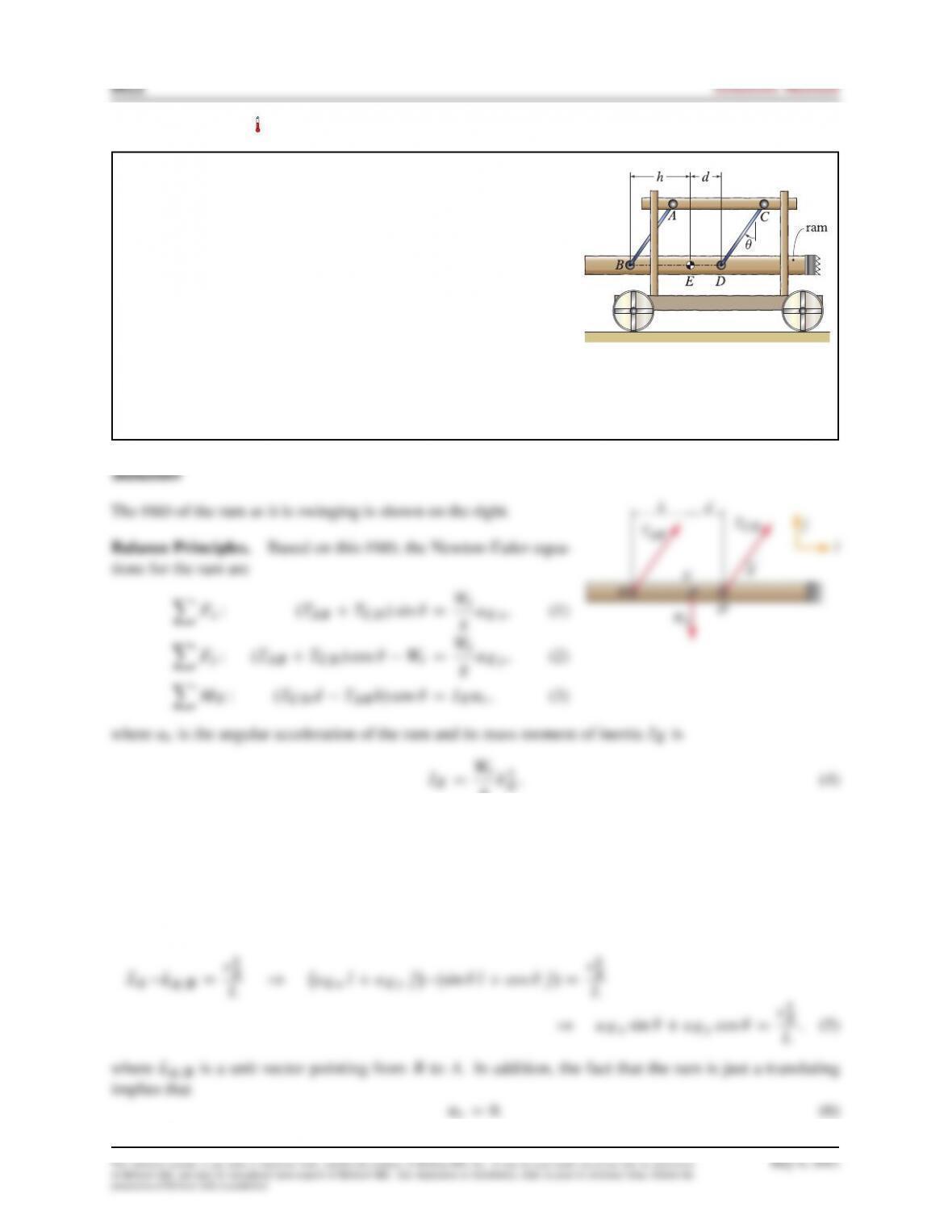
Problem 7.102
The figure shows a weapon called a battering ram (modern large
battering rams are typically mounted on armored vehicles). The
ram has a weight
WrD2500 lb
, center of mass at
E
, and radius of
gyration
kED6:5 ft
. Also let the distance between points
A
and
B
and between points
C
and
D
be
6ft
. In addition, let
hD4:5 ft
and
dD3ft
. Finally, let the connections at points
A
,
B
,
C
, and
D
be
pin connections, and assume that the cart does not move while the
ram swings.
Let the ram be at rest with
D0ı
. Assume that the cords
AB
and
CD
are inextensible and of negligible mass. Also assume that
cord
AB
breaks suddenly. Determine the tension in cord
CD
and
the acceleration of Eimmediately after AB breaks.
gk2
Force Laws. All forces have been accounted for on the FBD.
Kinematic Equations.
Since point
D
can only move in a circle centered at
C
, the acceleration of point
D
is of the form
EaDDaDx O{; (1)
of McGraw-Hill, and must be surrendered upon request of McGraw-Hill. Any duplication or distribution, either in print or electronic form, without the
permission of McGraw-Hill, is prohibited.
Dynamics 2e 1621
Computation.
Substituting the expressions for the mass moment of inertia and the kinematic equations
into the Newton-Euler equations, we obtain the following system of three equations in the three unknowns
gaDx; TCD WrD Wr
gd˛r;and TCD dDWr
gk2
the solution of which is
EWr
of McGraw-Hill, and must be surrendered upon request of McGraw-Hill. Any duplication or distribution, either in print or electronic form, without the
permission of McGraw-Hill, is prohibited.
Problem 7.103
The figure shows a weapon called a battering ram (modern large
battering rams are typically mounted on armored vehicles). The
ram has a weight
WrD2500 lb
, center of mass at
E
, and radius of
gyration
kED6:5 ft
. Also let the distance between points
A
and
B
and between points
C
and
D
be
6ft
. In addition, let
hD4:5 ft
and
dD3ft
. Finally, let the connections at points
A
,
B
,
C
, and
D
be
pin connections, and assume that the cart does not move while the
ram swings.
Assume that
AB
and
CD
are inextensible cords with negligible
mass. In addition, assume that, at the instant shown,
D10ı
and
the ram is swinging forward with
jEvEj D 7ft=s
. At this instant,
determine the acceleration of
E
, as well as the reaction forces at
points Aand C.
gk2
Force Laws. All forces have been accounted for on the FBD.
Kinematic Equations.
Since motion of the ram is a curvilinear translation, every point on it will have the
same velocity and same acceleration as every other point. Point
B
, for example, is moving in a circle centered
at
A
and so the component of the acceleration of
B
in the direction from
B
to
A
is
v2
E=L
, where
L
is the
length of the segment AB. Enforcing this condition, we obtain
E
E
of McGraw-Hill, and must be surrendered upon request of McGraw-Hill. Any duplication or distribution, either in print or electronic form, without the
permission of McGraw-Hill, is prohibited.
Dynamics 2e 1623
Computation.
After substituting the Eqs. (4) and (6) into Eqs. (1)–(3), the resulting three equations, along
with Eq. (5) gives the following system of four equations in the four unknowns aEx ,aEy ,TAB , and TCD
of McGraw-Hill, and must be surrendered upon request of McGraw-Hill. Any duplication or distribution, either in print or electronic form, without the
permission of McGraw-Hill, is prohibited.
Problem 7.104
The figure shows a weapon called a battering ram (modern large
battering rams are typically mounted on armored vehicles). The
ram has a weight
WrD2500 lb
, center of mass at
E
, and radius of
gyration
kED6:5 ft
. Also let the distance between points
A
and
B
and between points
C
and
D
be
6ft
. In addition, let
hD4:5 ft
and
dD3ft
. Finally, let the connections at points
A
,
B
,
C
, and
D
be
pin connections, and assume that the cart does not move while the
ram swings.
Assume that
AB
and
CD
are uniform thin rods weighing
100 lb
each. If the ram is released from rest when
D63ı
, determine the
acceleration of
E
, as well as the reaction forces at points
A
and
C
immediately after release.
gk2
is the mass moment of inertia of ram about its own mass center.
Based on the FBD of bar AB, its Newton-Euler equations are
2Lsin .AyCBy/1
2Lcos .AxCBx/DIG˛AB ;(7)
IGD1
12
gL2:(8)
of McGraw-Hill, and must be surrendered upon request of McGraw-Hill. Any duplication or distribution, either in print or electronic form, without the
permission of McGraw-Hill, is prohibited.
2Lsin .CyCDy/1
2Lcos .CxCDx/DIH˛CD;(11)
IHD1
12
gL2;(12)
Force Laws. All forces have been accounted for on the FBD.
Kinematic Equations.
Bars
AB
and
CD
are in fixed axis rotation about points
A
and
C
, respectively.
2.sin O{Ccos O|/DL
2˛bcos O{L
2˛bsin O| : (15)
Computation. Substituting Eqs. (4), (8), and (12)–(15) into the nine Newton-Euler equations we obtain
2g ˛bcos ; (19)
ByCAyWbD LWb
2g ˛bsin ; (20)
12g L2˛b;(24)
of McGraw-Hill, and must be surrendered upon request of McGraw-Hill. Any duplication or distribution, either in print or electronic form, without the
permission of McGraw-Hill, is prohibited.