Solutions to end–of–chapter problems
Engineering Economy, 7th edition
Leland Blank and Anthony Tarquin
Chapter 19
More on Variation and Decision Making Under Risk
19.1 (a) Continuous
(b) Discrete
19.2 (a) Discrete and Certainty
(b) Discrete and Risk
19.3 Needed or assumed information to calculate an expected value:
1. Treat output as discrete or continuous variable.
19.5 (a) Frequency distribution is as follows
Cell boundaries
Frequencies
19.5 – 31.5
4
31.5 – 43.5
10
43.5 – 55.5
8
55.5 – 67.5
6
67.5 – 79.5
3
(b) Probability distribution is as follows
Cell Boundaries
Frequencies
Probability
19.5 – 31.5
4
0.13
31.5 – 43.5
10
0.32
43.5 – 55.5
8
0.26
55.5 – 67.5
6
0.19
67.5 – 79.5
3
0.10
19.6 (a) N is discrete since only specific values are mentioned; i is continuous from 0 to 12.
(b) Plot the probability and cumulative probability values for N and i calculated below.
N 0 1 2 3 4__
(c) P(N = 1or 2) = P(N = 1) + P(N = 2)
= 0.56 + 0.26 = 0.82
19.7 (a) $ 0 2 5 10 100__
The variable $ is discrete, so plot $ versus F($).
3
(b) E($) = ∑$P($) = 0.91(0) + … + 0.007(100)
19.8 (a) P(N) = (0.5)N N = 1,2,3,…
N 1 2 3 4 5 etc.
19.9 First cost, P
PP = first cost to purchase
PL = first cost to lease
Use the uniform distribution relations in Equation [19.3] and plot.
Salvage value, S
SP is triangular with mode at $2500.
4
AOC AOCP is uniform with:
f(AOCL) is triangular with:
Life, L
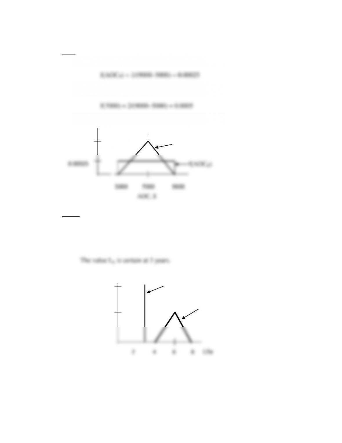
f(LP) is triangular with mode at 6:
f(6) = 2/(8-4) = 0.5
f(AOC
L
)
f(AOC)
0.5
1.0
f(LL)
f(LP)
f(L)
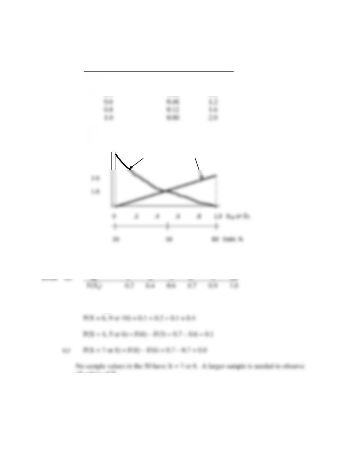
19.10 (a) Determine several values of DM and DY and plot.
DM or DY f(DM) f(DY)
0.0 3.00 0.0
0.2 1.92 0.4
0.4 1.08 0.8
f(DM) is a decreasing power curve and f(DY) is linear.
f(D)
f(DM) f(DY)
3.0
6
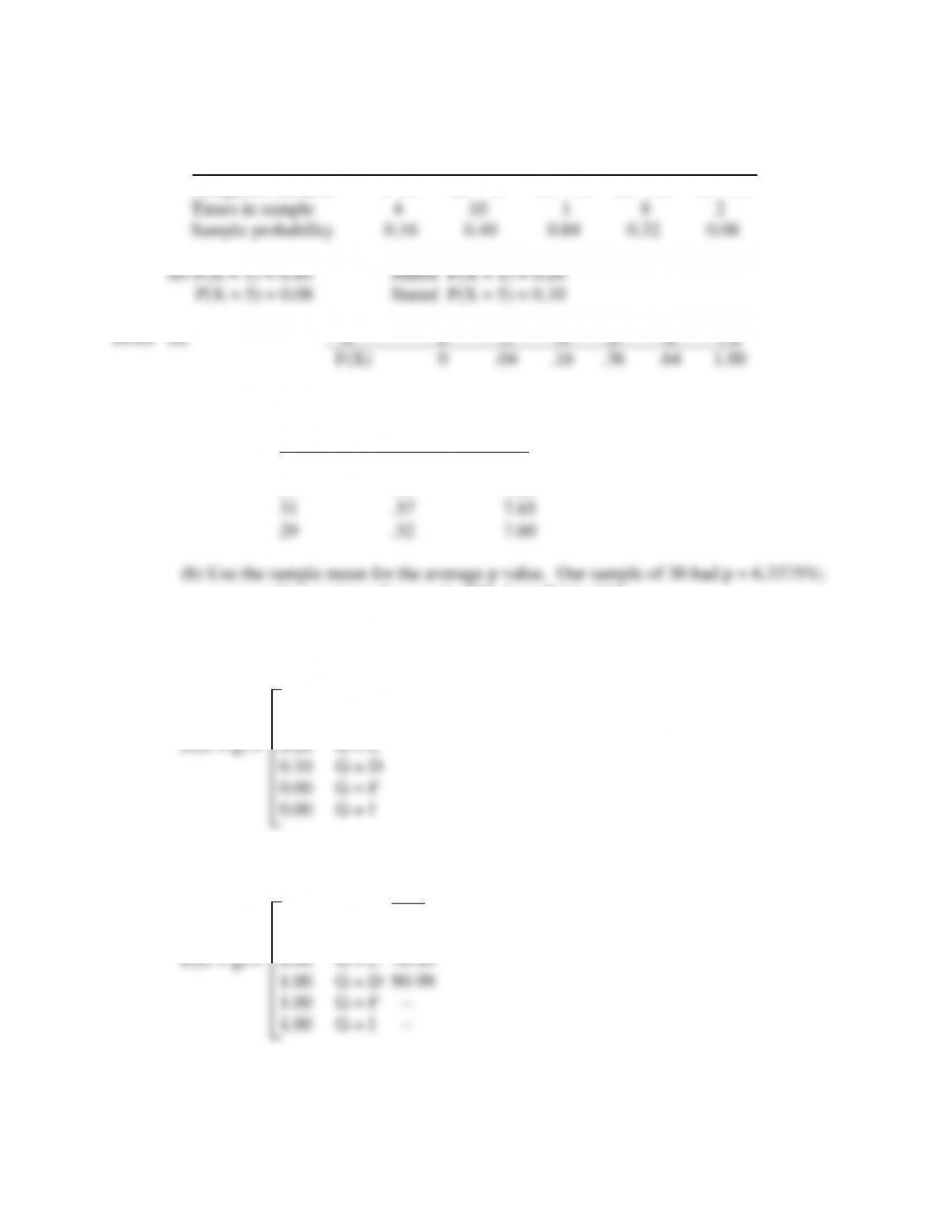
19.12 (a) Sample size is n = 25
Variable value 1 2 3 4 5
Assigned Numbers 0 -19 20 – 49 50 – 59 60 – 89 90 – 99
Take X and p values from the graph. Some samples are:
RN X p
18 .42 7.10%
59 .76 8.80
(b) Use the sample mean for the average p value. Our sample of 30 had p = 6.3375%;
yours will vary depending on the RNs from Table 19.2.
19.14 Use the steps in Section 19.3. As an illustration, assume the probabilities that are assigned
by a student are:
0.30 G = A
0.40 G = B
Steps 1 and 2: The F(G) and RN assignment are:
RNs
0.30 G = A 00-29
0.70 G = B 30-69
7
Steps 3 and 4: Develop a scheme for selecting the RNs from Table 19-2. Assume you
Step 5: Count the number of grades A through D, calculate the probability of each as
19.15 (a) When the RAND( ) function was used for 100 values in column A of a spreadsheet,
(b) For the RAND results, count the number of values in each cell to determine how
close it is to 10.
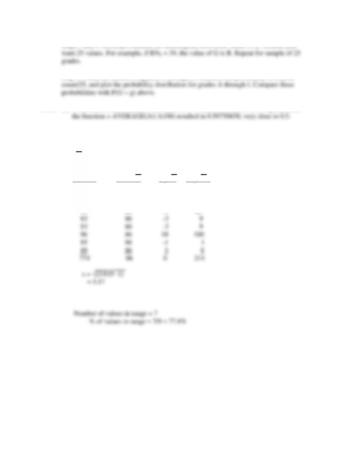
19.16 (a) X = (81, 86, 80, 91, 83, 83, 96, 85, 89)/9
= 86
(b) Reading Mean, X Xi – X (Xi – X)2
81 86 -5 25
86 86 0 0
80 86 -6 36
91 86 5 25
(c) Range for ±1s is 86 ± 5.17 = 80.83 – 91.17
8
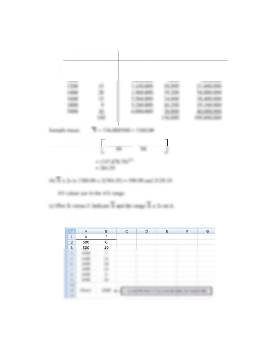
19.17 (a) Hand solution Use Equations [19.9] and [19.12].
Cell,
Xi fi Xi2 fiXi fiXi2
600 6 360,000 3,600 2,160,000
800 10 640,000 8,000 6,400,000
Std deviation: s = 199,600,000 – 100 (1360)2 1/2
(b) X ± 2s is 1360.00 ± 2(384.55) = 590.90 and 2129.10
(d) Use SUMPRODUCT and SUM functions to obtain average for frequency data.
9
19.18 (a) Convert P(X) data to frequency values to determine s.
X P(X) XP(X) f X2 fX2
1 .2 .2 10 1 10
2 .2 .4 10 4 40
(b) X ± 1s is 4.6 ± 3.42 = 1.18 and 8.02
19.19 (a) Use Equations [19.15] and [19.16]. Substitute Y for DY.
f(Y) = 2Y
1
Var(Y) = ∫ (Y2)2Ydy – [E(Y)]2
10
σ = (0.05556)0.5 = 0.236
1
P(0.195 ≤ Y ≤ 1.0) = ∫ 2Ydy
0.195
19.20 (a) Use Equations [19.15] and [19.16]. Substitute M for DM.
1
E(M) = ∫ (M) 3 (1 – M)2dm
(b) E(M) ± 2σ is 0.25 ± 2(0.1936) = –0.1372 and 0.6372
0.6372
P(0 ≤ M ≤ 0.6372) = ∫ 3(1 – M)2 dm
0
19.21 Use Equation [19.8] where P(N) = (0.5)N
E(N) = 1(.5) + 2(.25) + 3(.125) + 4(0.625) + 5(.03125) + 6(.015625) + 7(.0078125)
E(N) can be calculated for as many N values as you wish. The limit to the series N(0.5)N
is 2.0, the correct answer.
19.22 E(Y) = 3(1/3) + 7(1/4) + 10(1/3) + 12(1/12)
Var (Y) = ∑ Y2P(Y) – [E(Y)]2
E(Y) ± 1σ is 7.083 ± 3.227 = 3.856 and 10.310
19.23 Using a spreadsheet, the steps in Sec. 19.5 are applied.
1. CFAT given for years 0 through 6.
Col A: = RAND ( )* 100 to generate random numbers from 0-100.
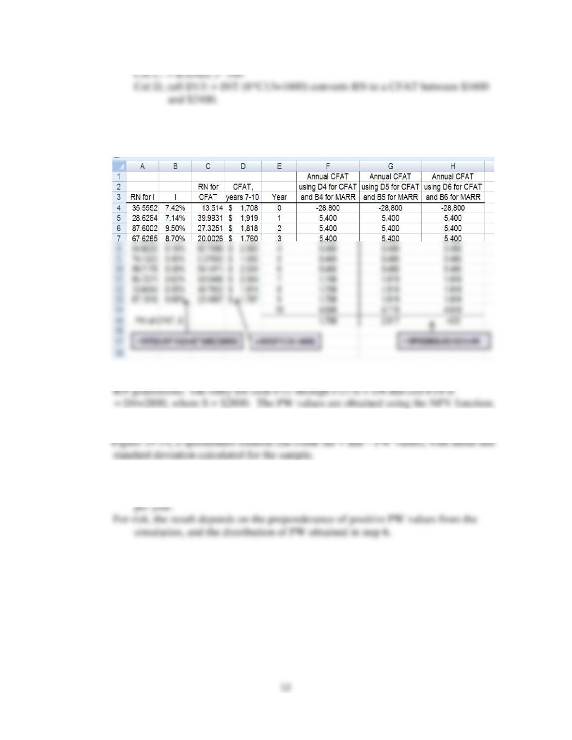
Ten samples of i and CFAT for years 7-10 are shown below in columns B and D
of the spreadsheet.
5. Columns F, G and H give 3 CFAT sequences, for example only, using rows 4, 5 and 6
6. Plot the PW values for as large a sample as desired. Or, following the logic of
7. Conclusion:
For certainty, accept the plan since PW = $2966 exceeds zero at an MARR of 7%
13
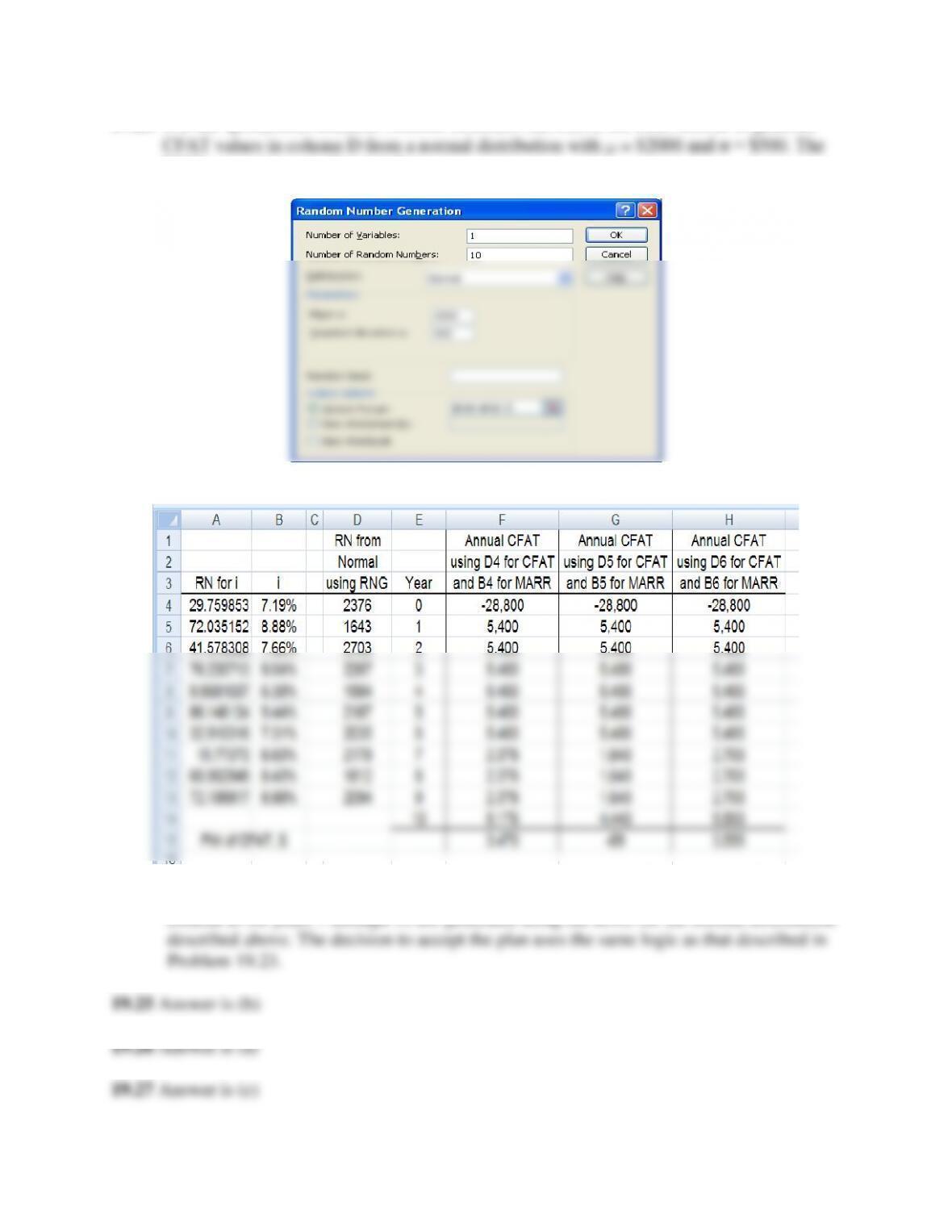
19.24 Use the spreadsheet Random Number Generator (RNG) on the tools toolbar to generate
RNG screen image is shown below.
The spreadsheet above is the same as that in Problem 19.23, except that CFAT values in
column D for years 7 through 10 are generated using the RNG for the normal distribution
14
19.29 P($ <9600) = P($ = 6200) + P($ = 8500)
19.32 Two numbers (46 and 27) are in the range 25 to 49, which indicate type B.

15
Solution to Case Study, Chapter 19
USING SIMULATION AND 3–ESTIMATE SENSITIVITY ANALYSIS
This simulation is left to the student. The 7-step procedure from Section 19.5 can be applied
here. Set up the RNG for the cash flow values of AOC, S, and n for each alternative. For each
sample cash flow series, calculate the AW value for each alternative. To obtain a final answer of