14
AW2.25 = –225,000(A/P,6%,10) + (–50,000)(0.1)
AW2.5 = –300,000(A/P,6%,10) + (–50,000)(0.05)
AW3.0 = –400,000(A/P,6%,10) + (–50,000)(0.01)
AW3.25 = –450,000(A/P,6%,10) + (–50,000)(0.005)
18.35 Compute the expected value for each outcome and select the maximum for D3.
Top node: 0.4(55) + 0.30(–30) + 0.30(10) = 16.0
15
18.36
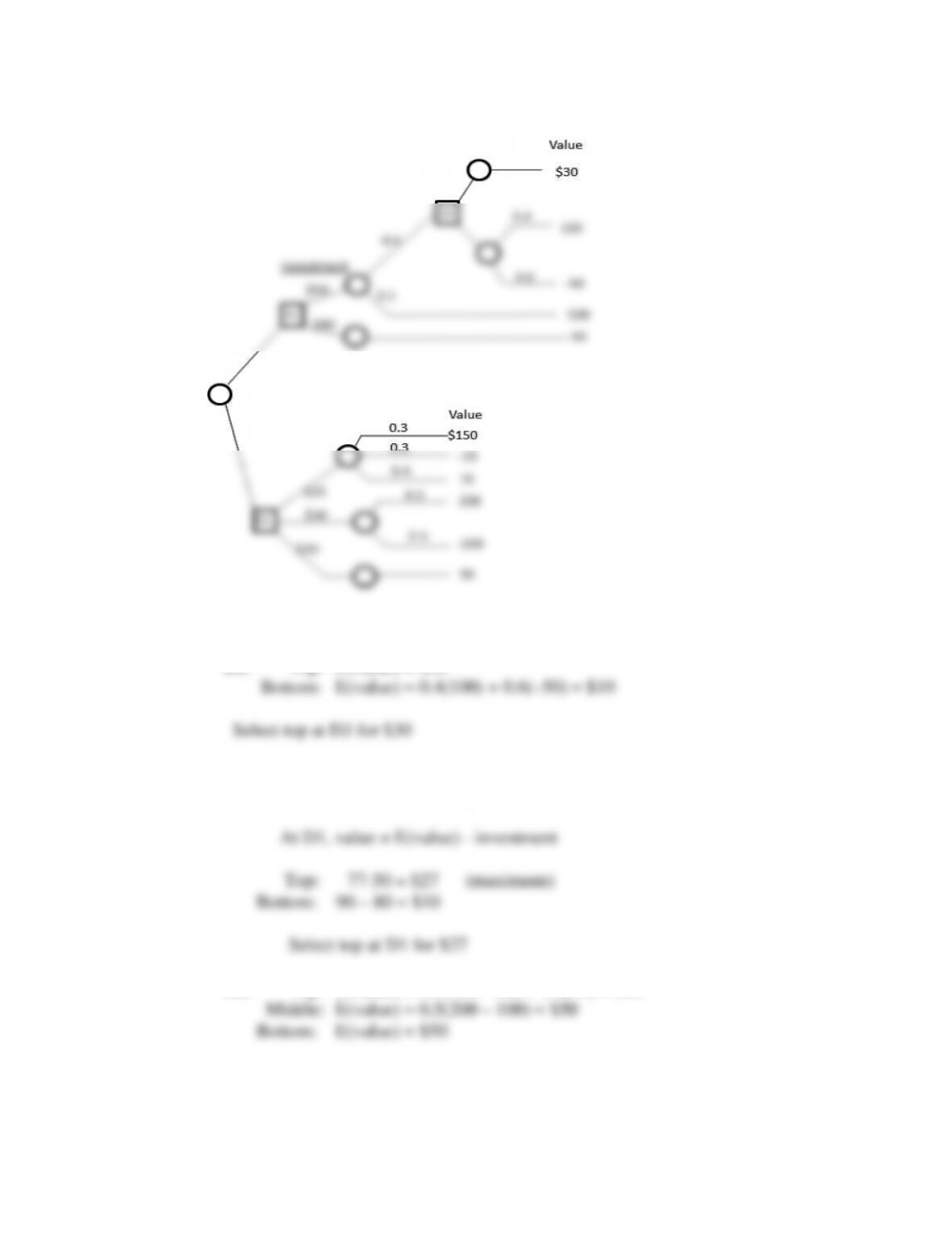
Maximize the value at each decision node.
D3: Top: E(value) = $30
D1: Top: 0.9(D3 value) + 0.1(final value)
0.9(30) + 0.1(500) = $77
D2: Top: E(value) = 0.3(150 – 30) + 0.4(75) = $66
16
At D2, value = E(value) – investment
18.37 Calculate the E(PW) in year 3 and select the largest expected value. In $1000 units,
E(PW of D4,x) = –200 + 0.7[50(P/A,15%,3)] + 0.3[40(P/F,15%,1)
E(PW of D4,z) = –350 + 0.7[190(P/A,15%,3) – 20(P/G,15%,3)]
17
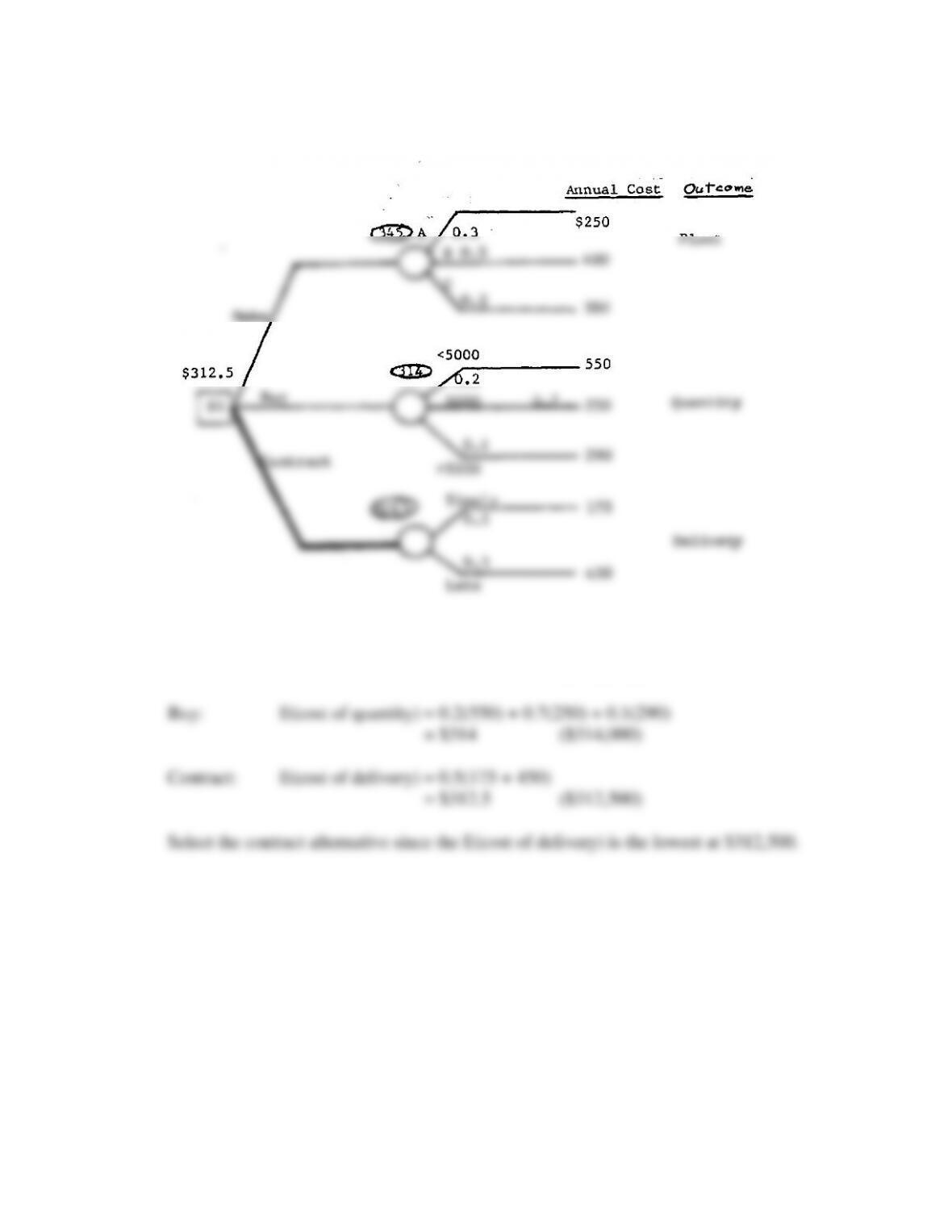
18.38 Select the minimum E(cost) alternative. All monetary units are times $-1000.
Make: E(cost of plant) = 0.3(250) + 0.5(400) + 0.2(350)
= $345 ($345,000)
18
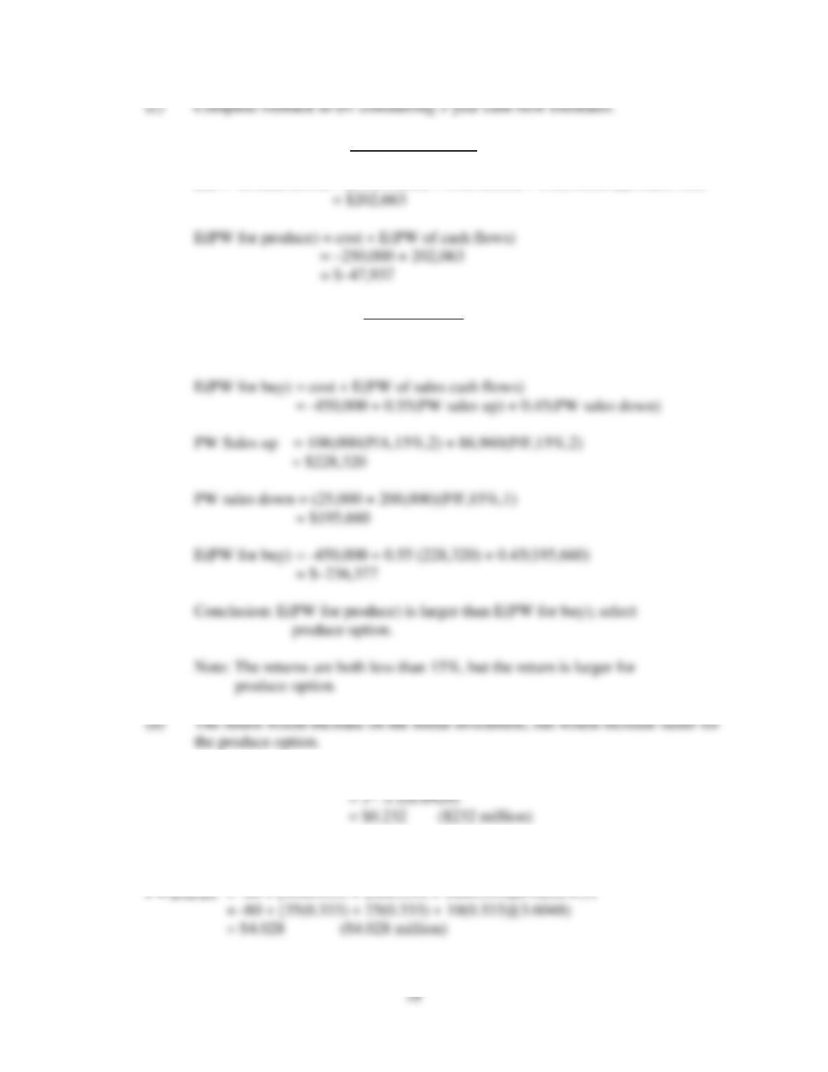
18.39 (a) Construct the decision tree.
(b) At D2 compute PW of cash flows and E(PW) using probability values.
Expansion option
(PW for D2, $120,000) = –100,000 + 120,000(P/F,15%,1)
No expansion option
(PW for D2, $100,000 = $100,000(P/F,15%,1) = $86,960
Produce option, D1
E(PW of cash flows) = [0.5(75,000) + 0.4(90,000) + 0.1(150,000](P/A,15%,3)
Buy option, D1
At D2, E(PW) = $86,960
18.40 In $ billion units, PWoption = 3 – 3.1(P/F,12%,1)
18.41 In $ million units,
20
PW1 year = -150,000 – 1,900,000(P/F,15%,1) + 1,000,000(0.70)(P/A,15%,5)(P/F,15%,1)
18.43 (a) Find E(PW) after determining E(Rt), the expected repair costs for each year t
E(R2) = 1/3(-500 -1000 –0) = $-500
21
22
Solutions to Case Studies, Chapter 18
Sometimes, there is not a definitive answer to a case study exercise. Here are example responses.
SENSITIVITY TO THE ECONOMIC ENVIRONMENT
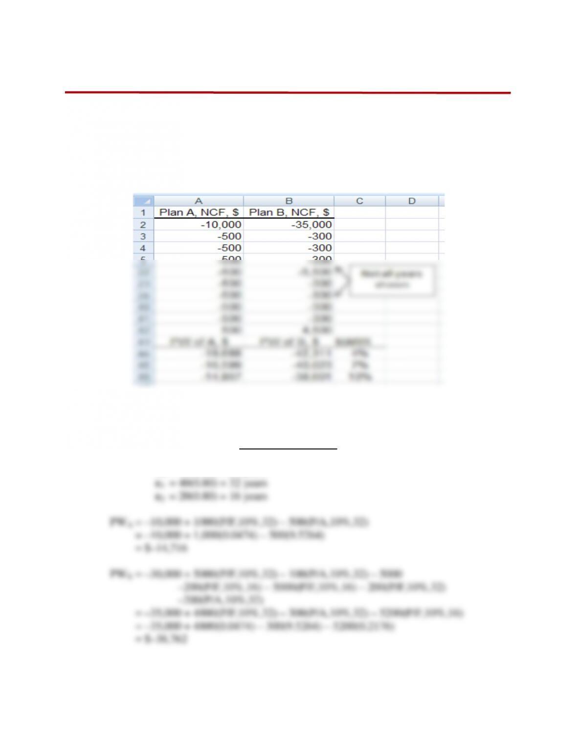
1. Spreadsheet analysis used for changes in MARR. PW is not very sensitive; plan A is
selected for all three MARR values.
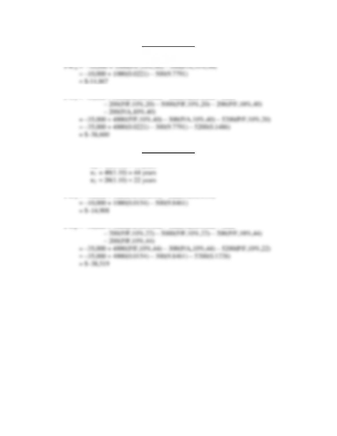
2. Sensitivity to changes in life is performed by hand. Not very sensitive; plan A has the best
PW for all life estimates.
Expanding economy
nA = 40(0.80) = 32 years
23
Expected economy
PWB = –30,000 + 5000(P/F,10%,40) – 100(P/A,10%,40) – 5000
Receding economy
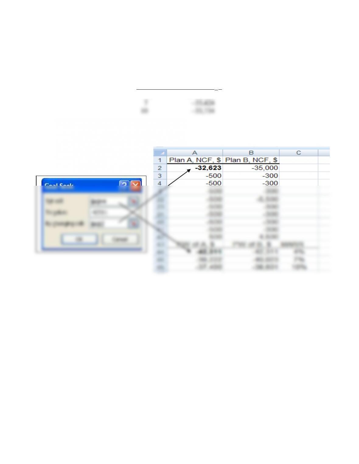
nA = 40(1.10) = 44 years
PWA = –10,000 + 1000(P/F,10%,44) – 500(P/A,10%,44)
PWB = –30,000 + 5000(P/F,10%,44) – 100(P/A,10%,44) – 5000
24
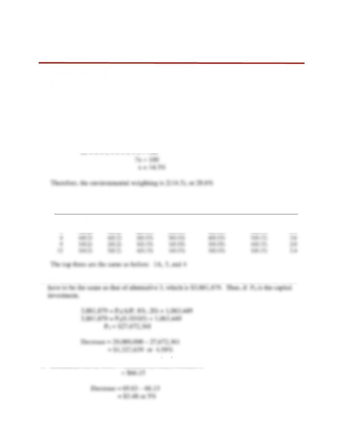
3. Use Goal Seek to find the breakeven values of PA
10% per year.
for the three MARR values of 4%, 7%, and
For MARR = 4%, the Goal Seek screen is below. Breakeven values are:
MARR Breakeven PA
4% $–32,623
_
The PA
breakeven value is not sensitive, but all three outcomes are over 3X the $10,000
estimated first cost for plan A.
25
Solutions to Case Studies, Chapter 18
Sometimes, there is not a definitive answer to a case study exercise. Here are example responses.
SENSITIVITY ANALYSIS OF PUBLIC SECTOR PROJECTS —
WATER SUPPLY PLANS
1. Let x = weighting per factor
Since there are 6 factors and one (environmental considerations) is to have a weighting that is
double the others, its weighting is 2x. Thus,
2.
Alt Ability to Relative Engineering Institutional Environmental Lead–Time
ID Supply Area Cost Feasibility Issues Considerations Requirement Total
1A 5(0.2) 4(0.2) 3(0.15) 4(0.15) 5(0.15) 3(0.15) 4.1
3. For alternative 4 to be as economically attractive as alternative 3, its total annual cost would
4. Household cost at 100% = 3,952,959(1/12)(1/4980)(1/1)
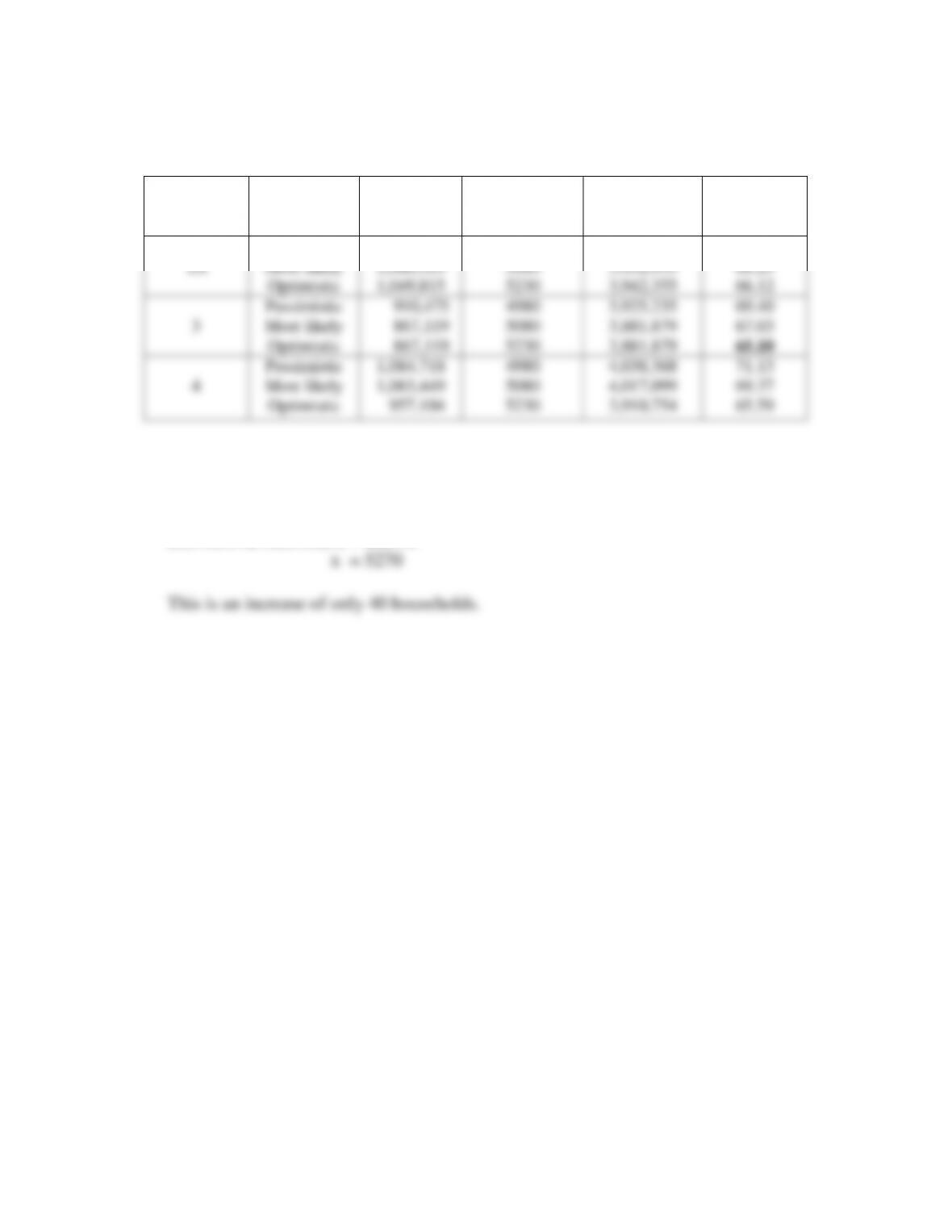
5. (a) Sensitivity analysis of M&O and number of households.
Alternative
Estimate
M&O,
$/year
Number of
households
Total
annual
cost, $/year
Household
cost,
$/month
Pessimistic
1,071,023
4980
3,963,563
69.82
Pessimistic
910,475
4980
3,925,235
69.40