1
Solutions to end–of–chapter problems
Engineering Economy, 7th edition
Leland Blank and Anthony Tarquin
Chapter 18
Sensitivity Analysis and Staged Decisions
18.1 $135,000: PW = -500,000 + 135,000(P/A,15%,5)
18.2 Start family now: FW = 50,000(F/A,10%, 5)(F/P,10%,20) + 15,000(F/A,10%,20)
Their retirement goal is not sensitive to when they start their family.
18.3 Invest now: FW = -80,000(F/P,20%,6) + 25,000(F/A,20%,6)
Invest 1–year from now: FW = -80,000(F/P,20%,5) + 26,000(F/A,20%,5)
The timing will affect whether the company earns its MARR; invest now.
18.4 Low pressure: A = 465 + 0.67(3,000,000/1000) = $2475 per day
2
18.5 AWcurrent = $-63,000
AW10,000 = -64,000(A/P,15%,3) – 38,000 + 10,000(A/F,15%,3)
AW18,000 = -64,000(A/P,15%,3) – 38,000 + 18,000(A/F,15%,3)
18.6 Joe: PW = –77,000 + 10,000(P/F,8%,6) + 10,000(P/A,8%,6)
Jane: PW = –77,000 + 10,000(P/F,8%,6) + 14,000(P/A,8%,6)
18.7 AWCnt = $-175,000
AWHigh = -250,000(A/P,15%,3) -75,000 + 90,000(A/F,15%,3)
18.8 Required AW < $5.7 million
10%: AW = -10,500,000(A/P,10%,5) – 3,100,000 + 2,000,000(A/F,10%,5)
18.9 AWCont = -130,000(A/P,15%,5) -30,000 + 40,000(A/F,15%,5)
18.10 (a) Q = FC/(70-40) = FC/30
_FC, $ QBE, units
200,000 6667
250,000 8333
18.11 PW = –P + (60,000 – 5000)(P/A,10%,5)
Percent
variation
P value, $
PW, $
-25%
-150,000
58,494
-20 -160,000 48,494
-200,000
8,494
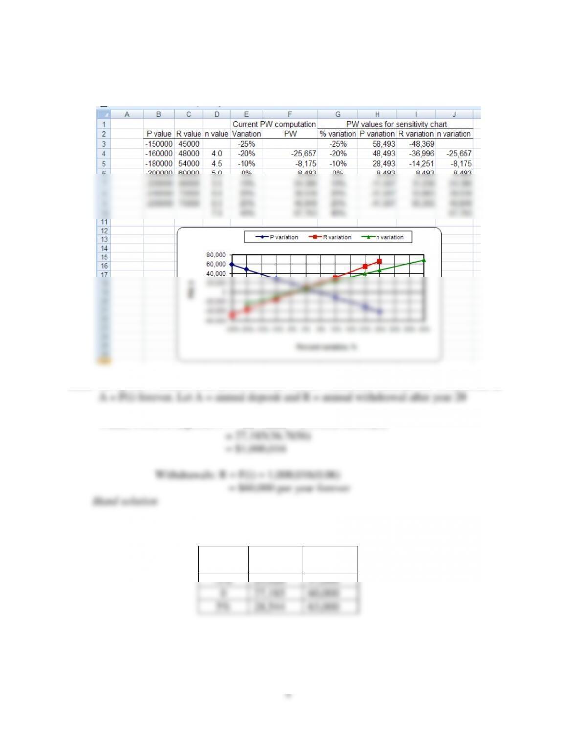
18.14 Spreadsheet is plotted for all three parameters: P. R and n. Variations in P and R have
about the same effect on PW in opposite directions, and more effect than variation in n.
18.15 Set up the F relation in 20 years, consider this a P value, and calculate the withdrawals at
Future worth of deposits: F = A(F/A,i,n) = 27,185(F/A,6%,20)
(a) R = A(F/A,6%,20)(i) = A(36.7856)(0.06)
Percent
variation
A, annual
deposit, $
R,
$ per year
-5%
25,826
57,000
0
27,185
60,000
5%
28,544
63,000
6
Return
value
Percent
variation
R,
$ per year
5%
-16.7%
44,945
6%
0
60,000
7%
16.7%
78,012
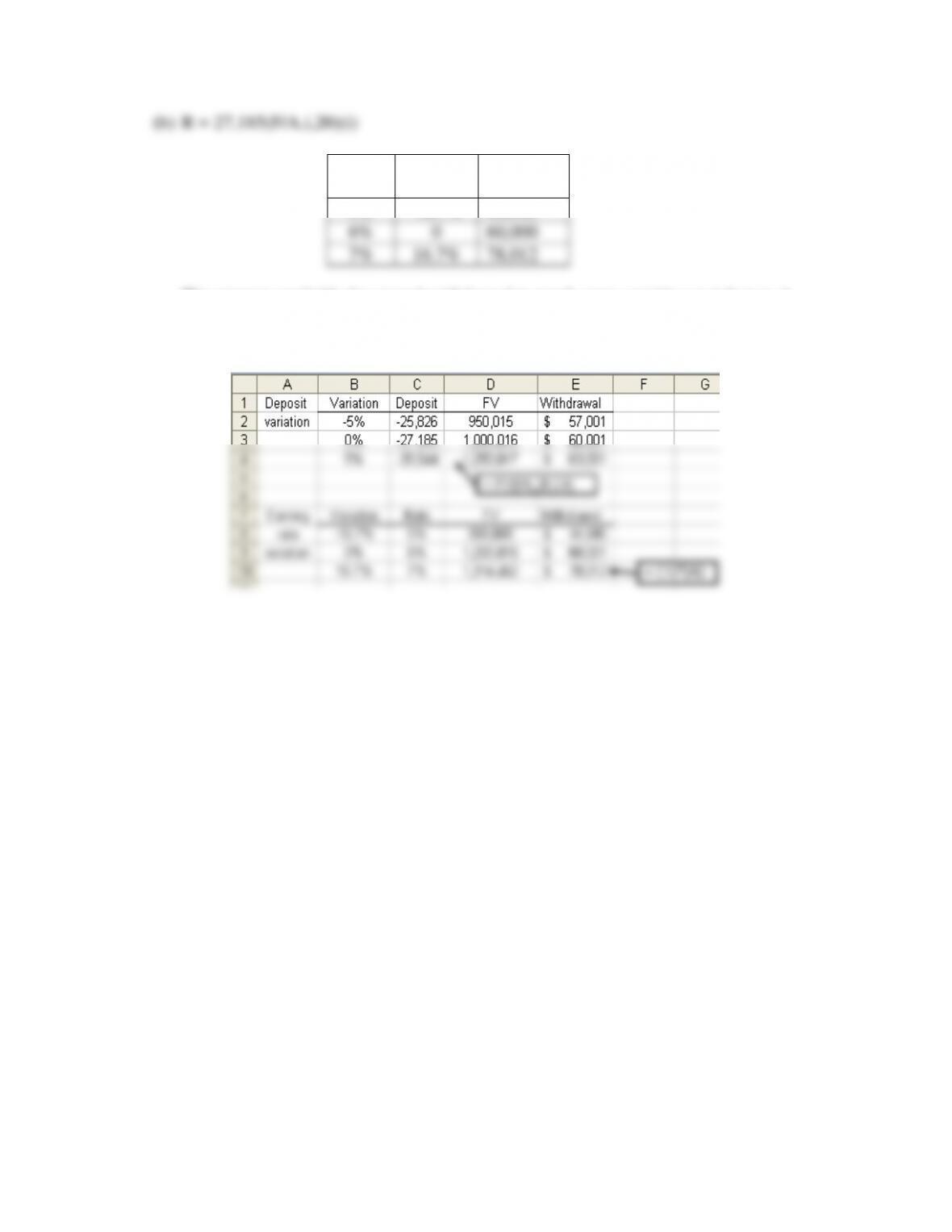
The amount available for annual withdrawal is much more sensitive to i than to A.
Spreadsheet solution
7
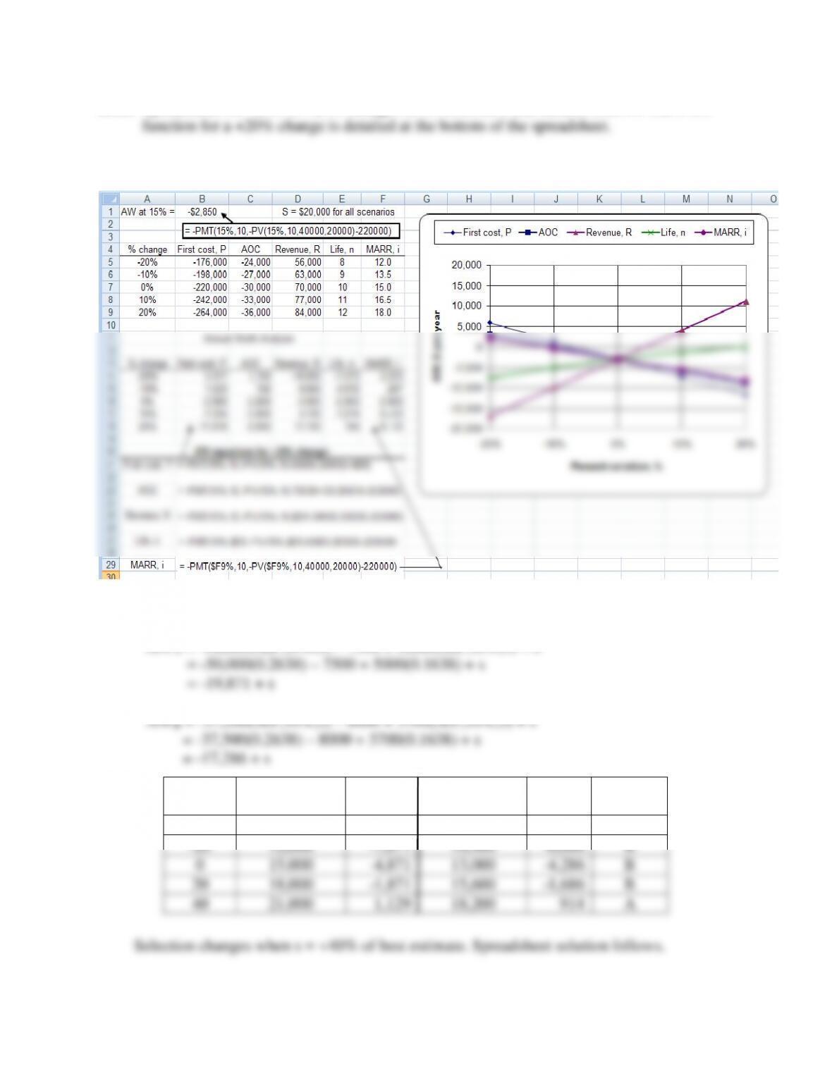
18.16 Spreadsheet for -20% to +20% changes in P, AOC, R, n and MARR follows. The PMT
AW is most sensitive to variations in revenue R and least sensitive to variations in life n.
18.17 Determine AW values at different savings, s.
AWA = -50,000(A/P,10%,5) – 7500 + 5,000(A/F,10%,5) + s
0
15,000
-4,871
13,000
-4,286
B
18,000
-1,871
15,600
-1,686
B
21,000
1,129
18,200
914
A
Percent
variation
Savings for A,
$ per year
AWA
Savings for B,
$ per year
AWB
Selection
-40%
9,000
$-10,871
7,800
$-9,486
B
-20
12,000
-7,871
10,400
-6,886
B
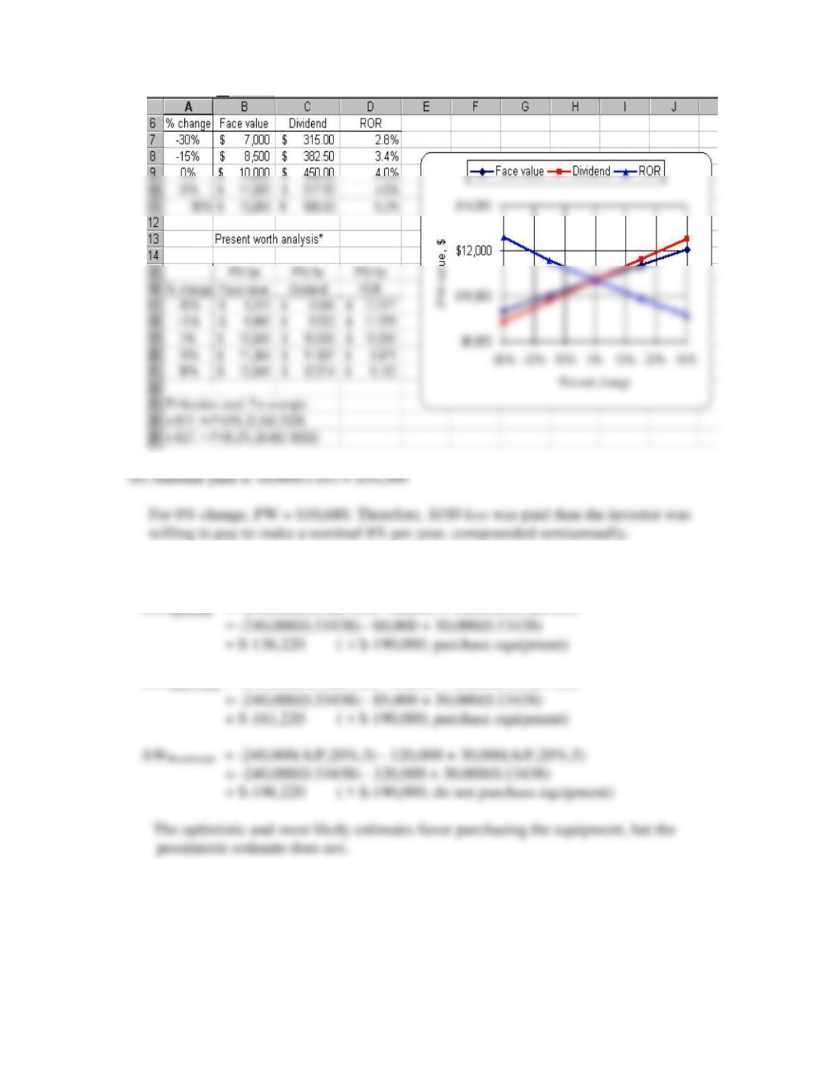
(1) Face value, V
(2) Dividend rate, b
(3) Nominal rate, r
9
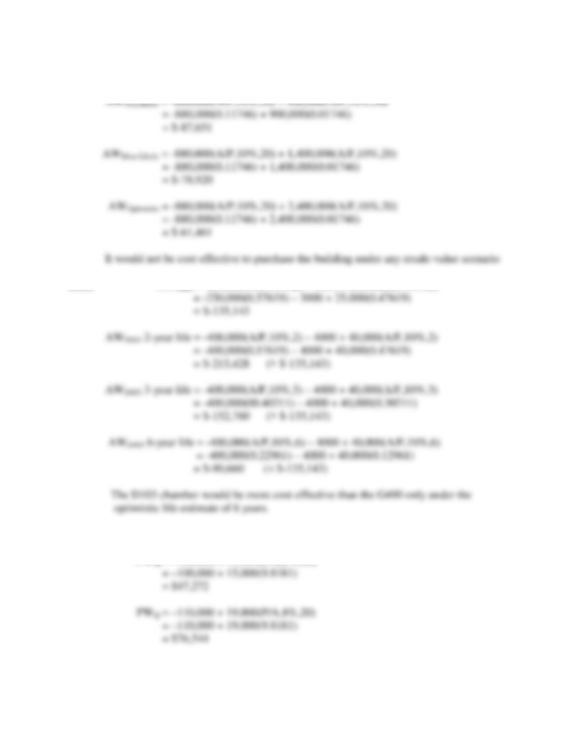
18.19 AWContract = $-190,000
AWOptimistic = -240,000(A/P,20%,5) – 60,000 + 30,000(A/F,20%,5)
AWMost Likely = -240,000(A/P,20%,5) – 85,000 + 30,000(A/F,20%,5)
10
18.20 AWLease = $-30,000 per year
18.21 AW490G = -250,000(A/P,10%,2) – 3000 + 25,000(A/F,10%,2)
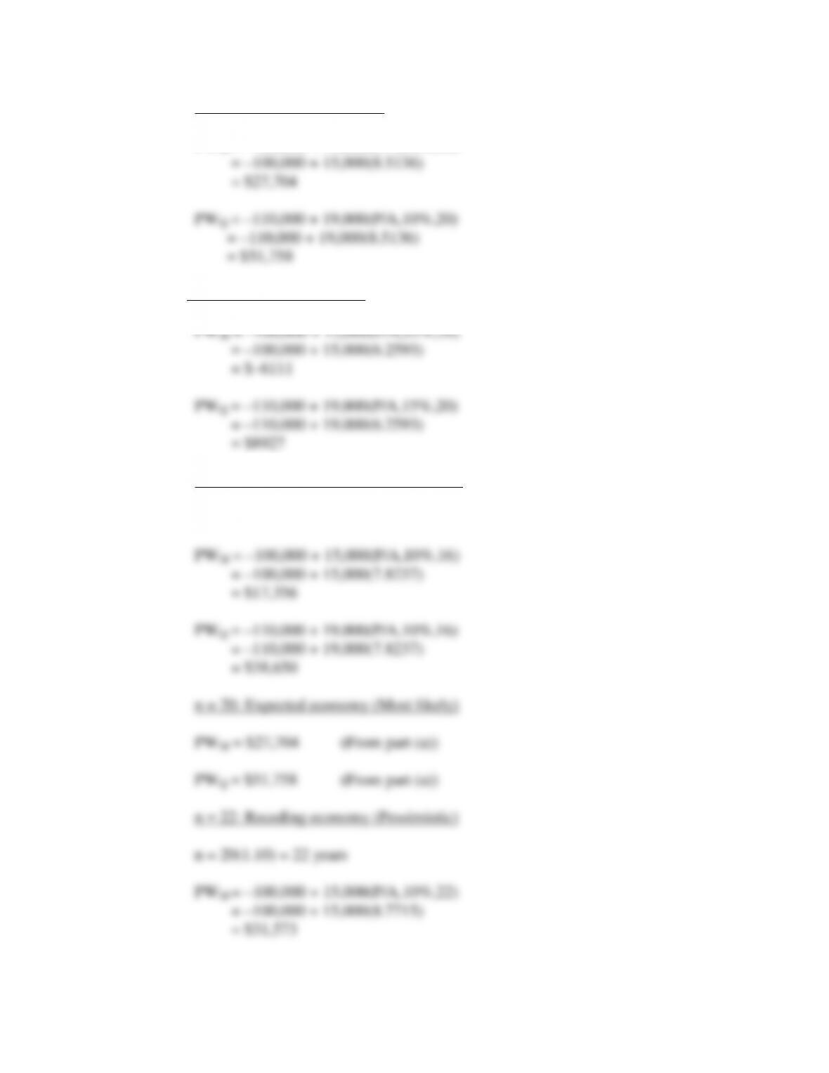
18.22 (a) MARR = 8% (Pessimistic)
PWM = –100,000 + 15,000(P/A,8%,20)
11
MARR = 10% (Most Likely)
PWM = –100,000 + 15,000(P/A,10%,20)
MARR = 15% (Optimistic)
(b)
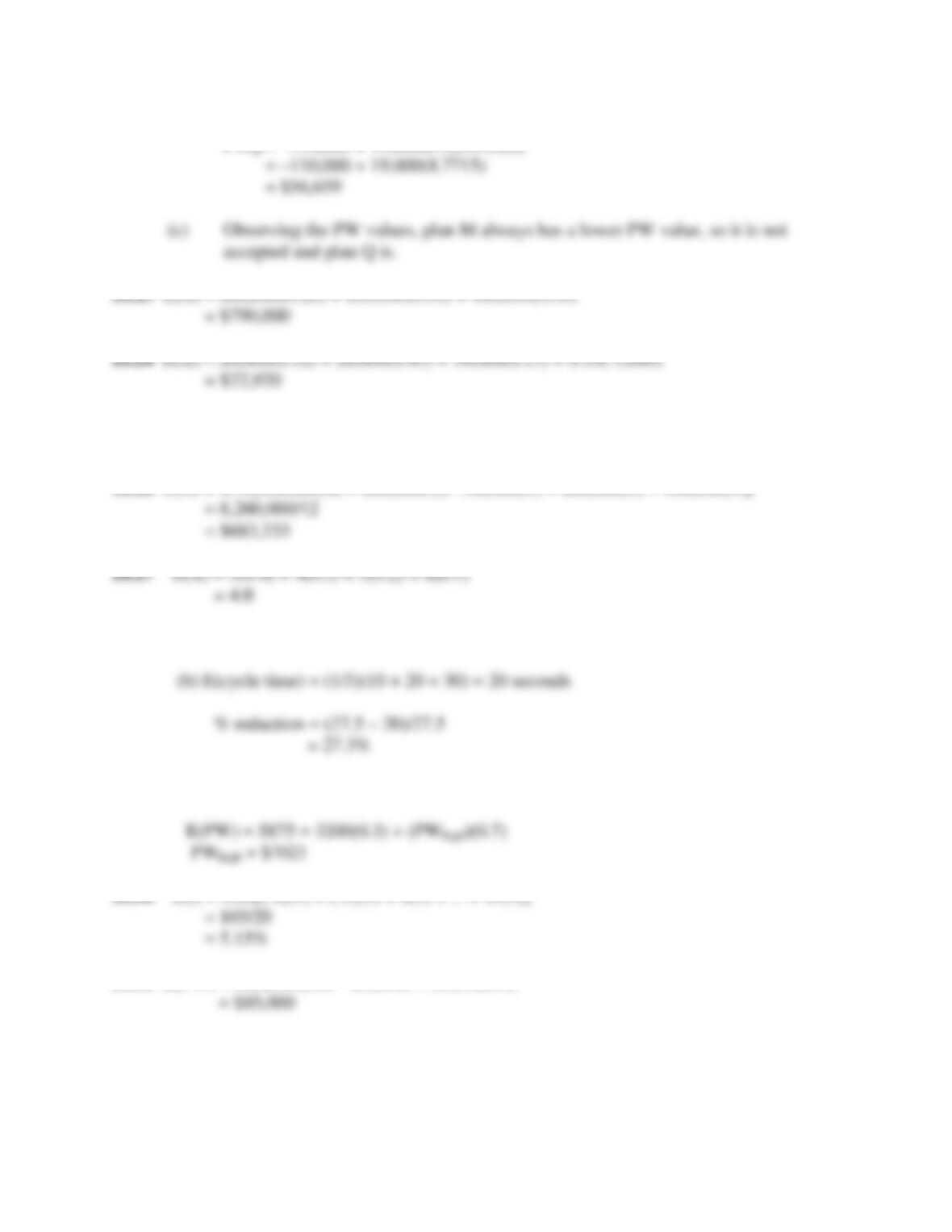
n = 16: Expanding economy (Optimistic)
n = 20(0.80) = 16 years
12
PWQ = –110,000 + 19,000(P/A,10%,22)
18.25 E(X) = (0.13)[1,500,000 + 1,900,000 + 2,400,000)]/3
= $251,333
18.26 E(X) = 1/12[500,000(4) + 600,000(2)+ 700,000(1) + 800,000(2) + 900,000(3)]
18.28 (a) E(cycle time) = (1/4)(10 + 20 + 30 + 50) = 27.5 seconds
18.29 Solve for PWhigh from E(PW)
18.30 E(i) = 1/20[(-8)(1) + (-5)(1) + 0(5) + … + 15(3)]
18.31 E(FW) = 0.20(300,000 – 25,000) + 0.6(50,000)
13
18.32 Determine E(AW) after calculating E(revenue).
E(revenue) = [days)(climbers)(income/climber)](probability)
E(AW) = –375,000(A/P,12%,10) – 25,000[(P/F,12%,4) + (P/F,12%,8)]
18.33 Determine E(PW) after calculating the PW of E(revenue)
E(revenue) = P(slump)(revenue over 3–year periods)
PW[E(revenue)] = PW[P(slump)(revenue 1st 3 years)
E(PW) = -200,000 + 200,000(0.12) (P/F,8%,6) + PW[E(revenue)]
18.34 AW = annual loan payment + (damage) × P(rainfall amount or greater)
Subscript on AW indicates rainfall amount.