1
Solutions to end–of–chapter problems
Engineering Economy, 7th edition
Leland Blank and Anthony Tarquin
Chapter 13
Breakeven and Payback Analysis
13.1 (a) 0 = -FC + (589 – 340)9000
13.2 (a) QBE = 800,000/(2950 – 2075)
13.3 Let r = selling price per pound of recovered metals
13.4 France: QBE = 3.5 million/(8500-3900)
13.5 France: QBE = 761 = 3.5million (1.10)/(r – 3900)
r = 3.85 million/761 + 3900
13.6 France: Profit = 8500(950) – 3,500,000 – 3900(950)
2
13.7 France: Profit = 1,000,000 = 8500(950) – 3,500,000 –v(950)
13.8 Gasoline required at 25.5 mpg = 1000/25.5 = 39.2 gallons
Gasoline required at 35.5 mpg = 1000/35.5 = 28.2 gallons
13.9 (a) QBE = 775,000 = 516,667 calls per year
2.50 – 1
3
13.10 Let m = miles driven per month to break even
Gasoline cost savings = 3.25/18 – 3.25/21 = $0.0258/mile
13.11 Added income for equipment from extra charges is
1421 – 758 – 400 = $263 per patient
13.12 Current cost per mile = 3.50/20 = $0.175 per mile
13.13 [2.90/18]x miles = (2.98 – 2.90)20
13.14 Let G = gradient increase per year. Set revenue = cost
[4000 + G(A/G,12%,3)](33,000 – 21,000) = -200,000,000(A/P,12%,3)
4
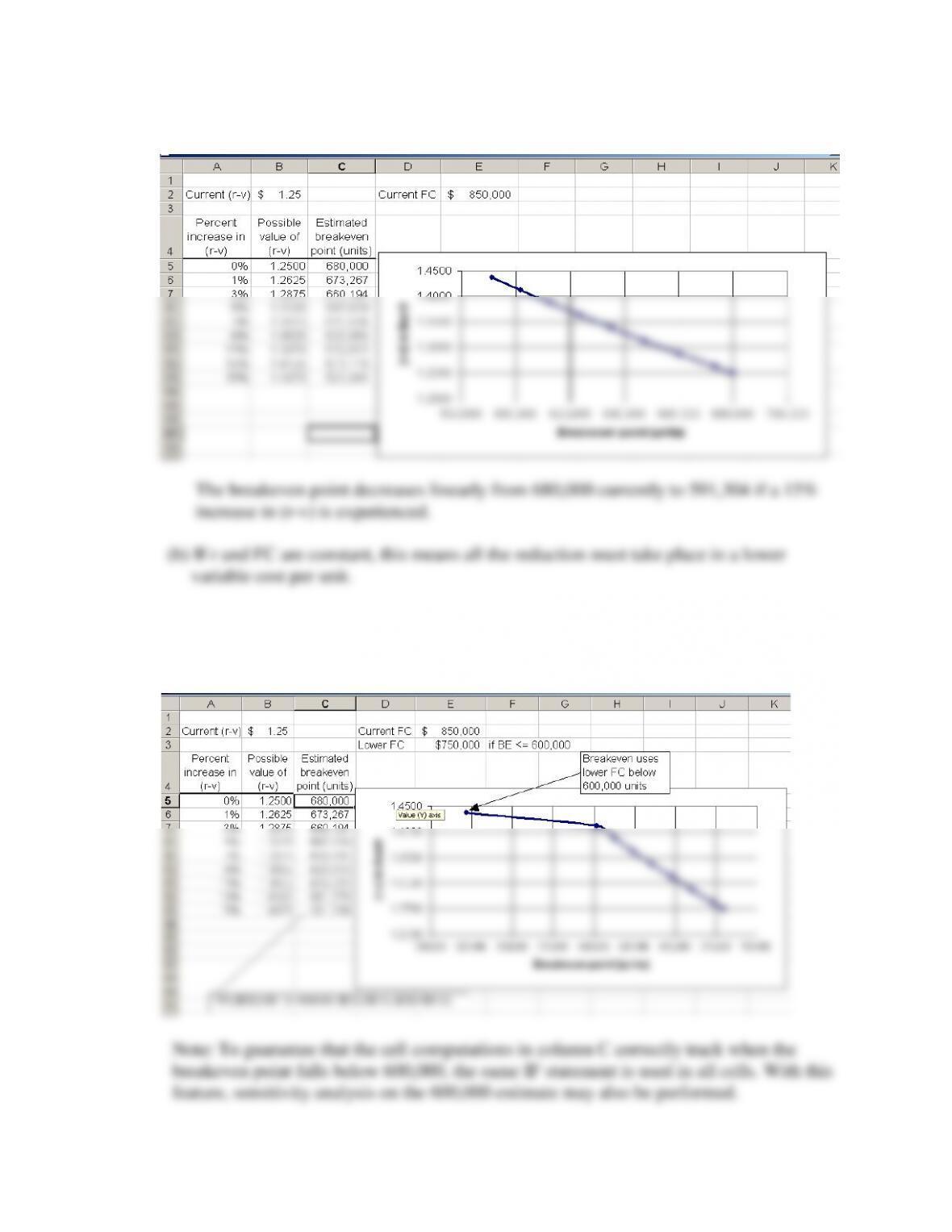
13.15 (a) Calculate QBE = FC/(r–v) for (r-v) increases of 1% through 15% and plot.
13.16 Rework the spreadsheet above to include an IF statement for the computation of QBE for
the reduced FC of $750,000. The breakeven point falls substantially to 521,739 when the
lower FC is in effect.
5
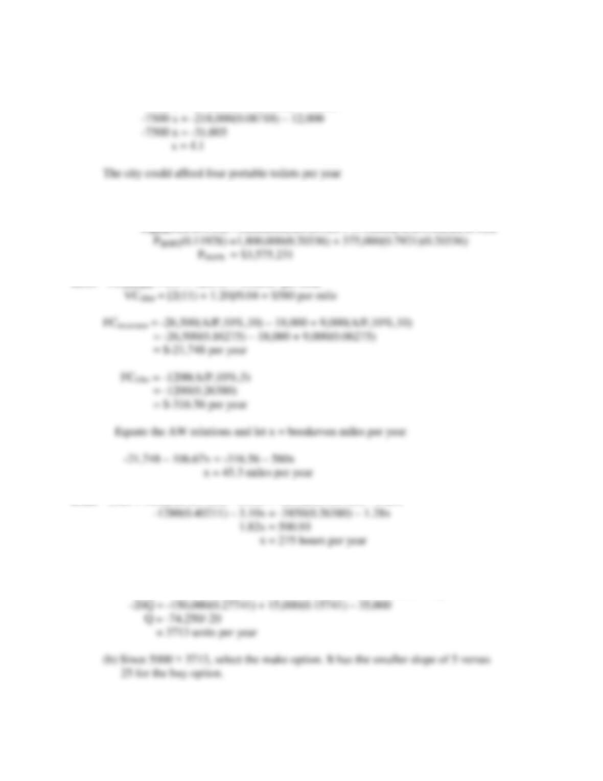
13.17 Let x = number of portables per year
-7500 x = -218,000(A/P,6%,20) – 12,000
13.18 Equate AW relations for the two alternatives
PHDPE(A/P,6%,12) =1,800,000(A/P,6%,6) + 375,000(P/F,6%,4)(A/P,6%,6)
13.19 VCexcavator = (15 + 1)/0.15 = $106.67 per mile
13.20 -(920 + 360)(A/P,10%,3) – 3.10x = -3850(A/P,10%,5) – 1.28x
13.21 (a) Solve the relation AWbuy = AWmake for Q = number of units per year.
-25Q = -150,000(A/P,12%,5) + 15,000(A/F,12%,5) – 35,000 – 5Q
6
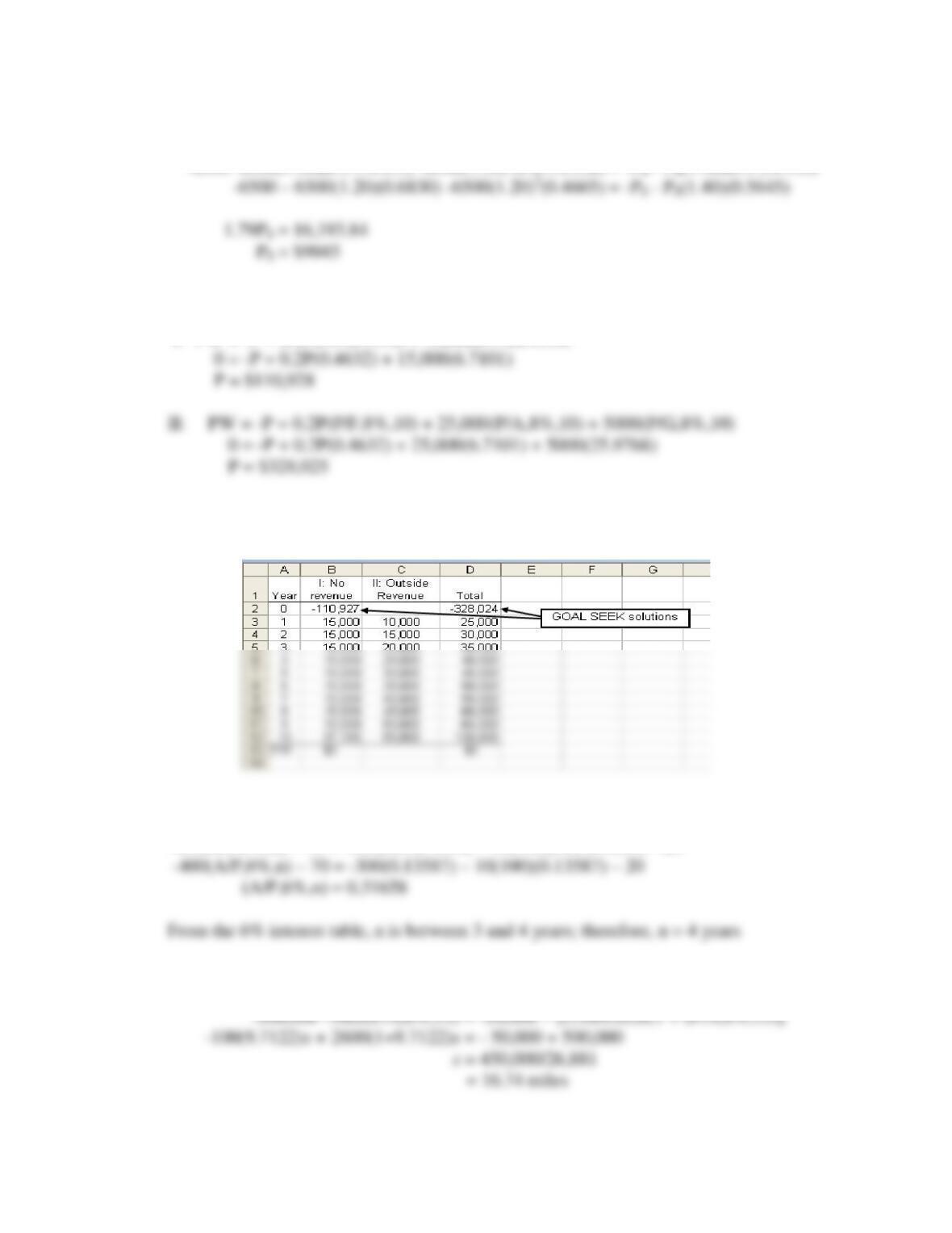
13.22 Equate PW relations; solve for PS. Painting and blasting is not done at end of year 12.
-6500 -6500(1.20)(P/F,10%,4) -6500(1.20)2(P/F,10%,8) = -PS – PS(1.40)(P/F,10%,6)
13.23 (a) Develop PW = 0 relation and solve for first cost P.
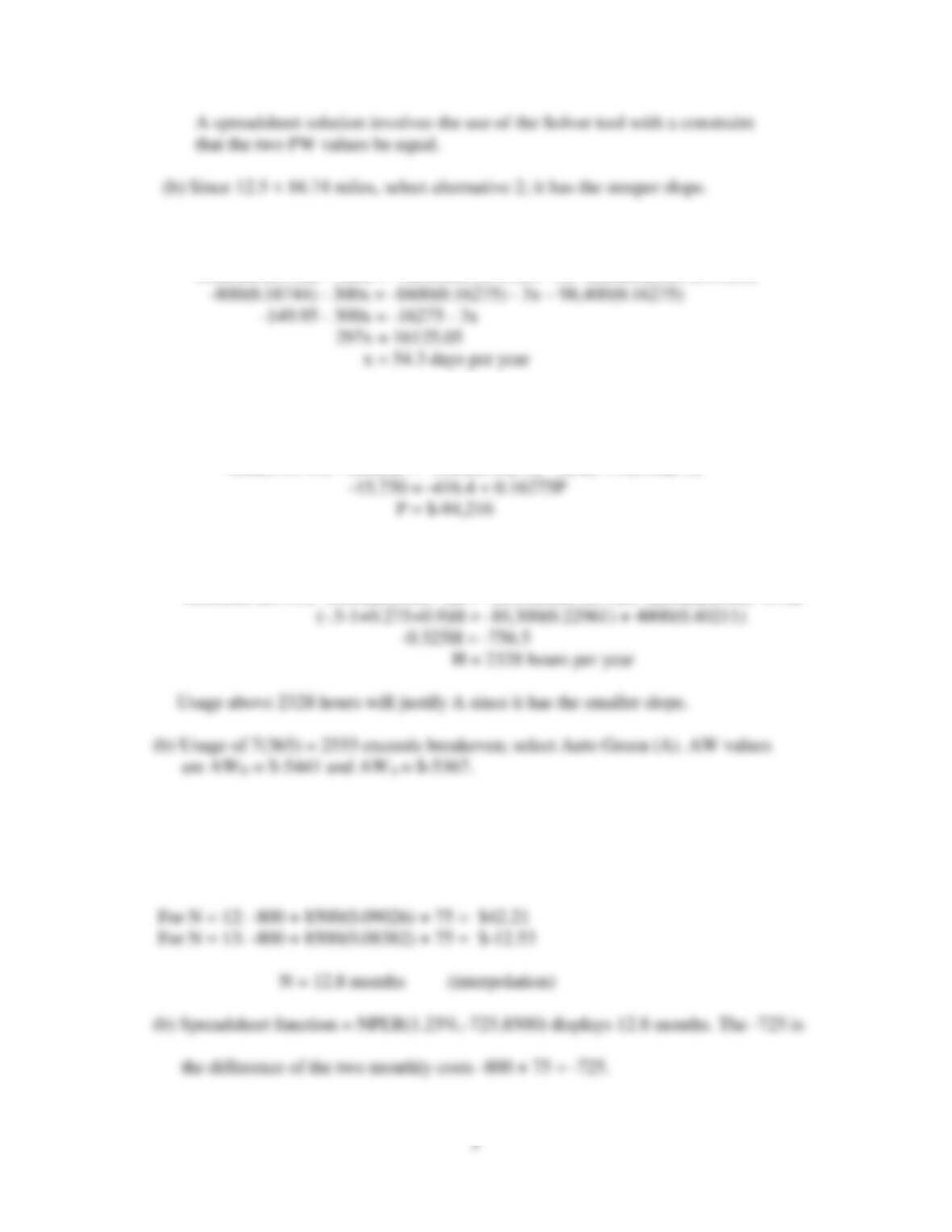
I: PW = -P + 0.2P(P/F,8%,10) + 15,000(P/A,8%,10)
(b) Spreadsheet solution uses Goal Seek to find P for each scenario.
13.24 Let x = number of years for above-ground pool to last for break even
-400(A/P,6%,n) – 70 = -300(A/P,6%,10) – 10(100)(A/P,6%,10) – 20
13.25 (a) Solve the relation PW1 = PW2 for x miles
13.26 (a) Let x = days per year to pump the lagoon. Set the AW relations equal.
-800(A/P,10%,8) – 300x = -1600(A/P,10%,10) – 3x -12(8200)(A/P,10%,10)
(b) If the lagoon is pumped 52 times per year and P = cost of pipeline, the breakeven
equation becomes:
-800(0.18744) – 300(52) = -1600(0.16275) – 3(52) + P(0.16275)
13.27 (a) Solve the relation AWN = AWA for H = number of hours per year.
-4000(A/P,10%,3) -1000(H/2000) –1H = -10,300(A/P,10%,6) -2200(H/8000) -0.9H
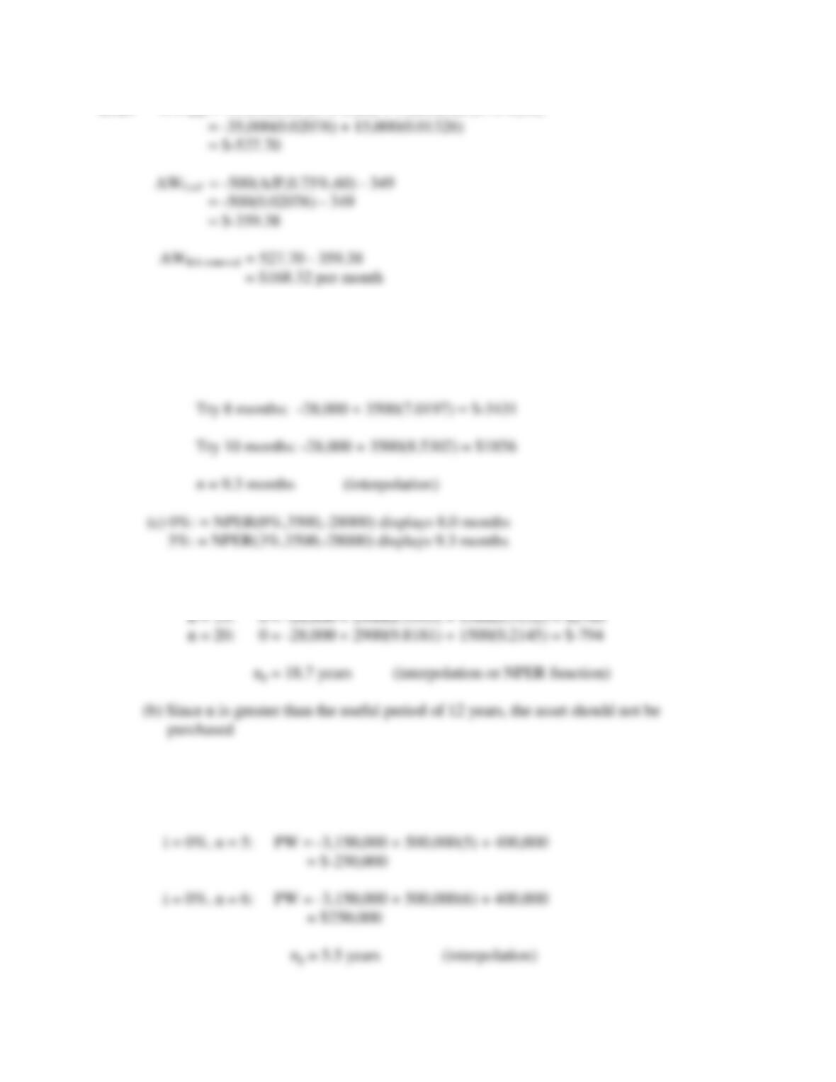
13.28 (a) Solve the relation AWlease – AWbuy = 0 for N = number of months
Monthly i = 1.25%.
-800 + 8500(A/P,1.25%,N) + 75 = 0
8
13.29 AWVolt = -35,000(A/P,0.75%,60) + 15,000(A/F,0.75%,60)
13.30 (a) np = 28,000/(5000-1500)
= 8 months
(b) 0 = -28,000 + (5000 – 1500)(P/A,3%,np)
13.31 (a) 0 = -28,000 + 2900(P/A,8%,n) + 1500(P/F,8%,n)
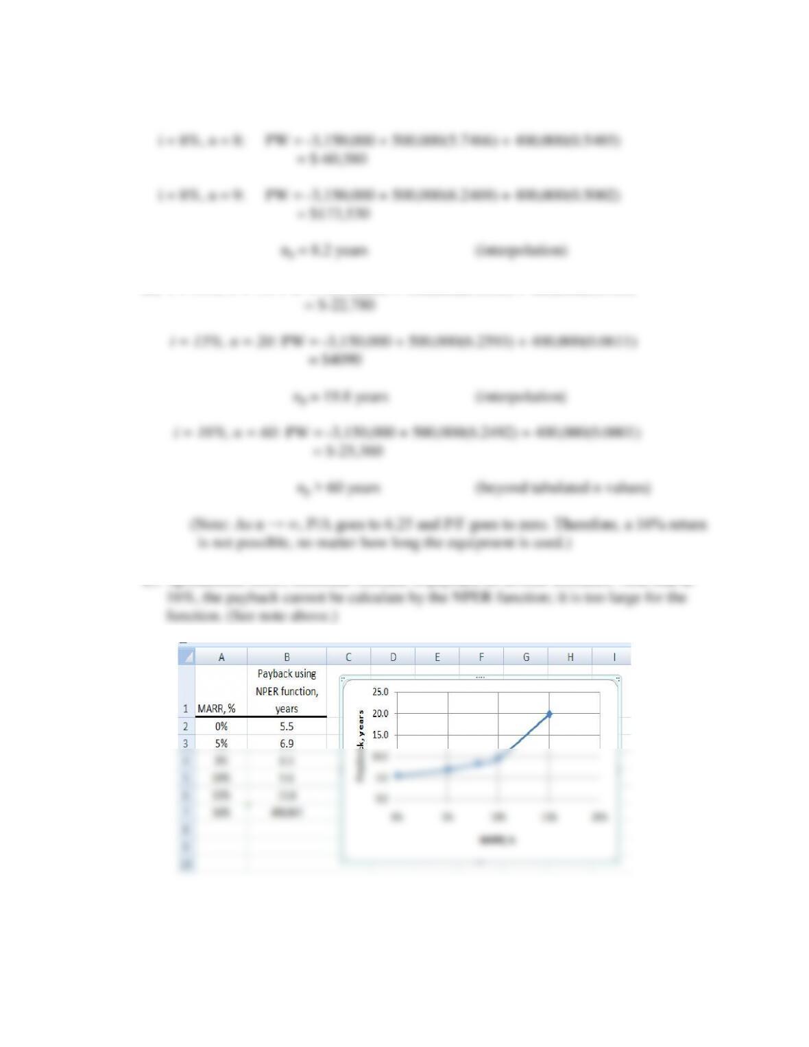
13.32 (a) Set PW = 0 at given interest rates and solve for np
0 = -3,150,000 + 500,000(P/A,i%,np) + 400,000(P/F,i%,np)
9
(b) i = 15%, n = 19: PW = -3,150,000 + 500,000(6.1982) + 400,000(0.0703)
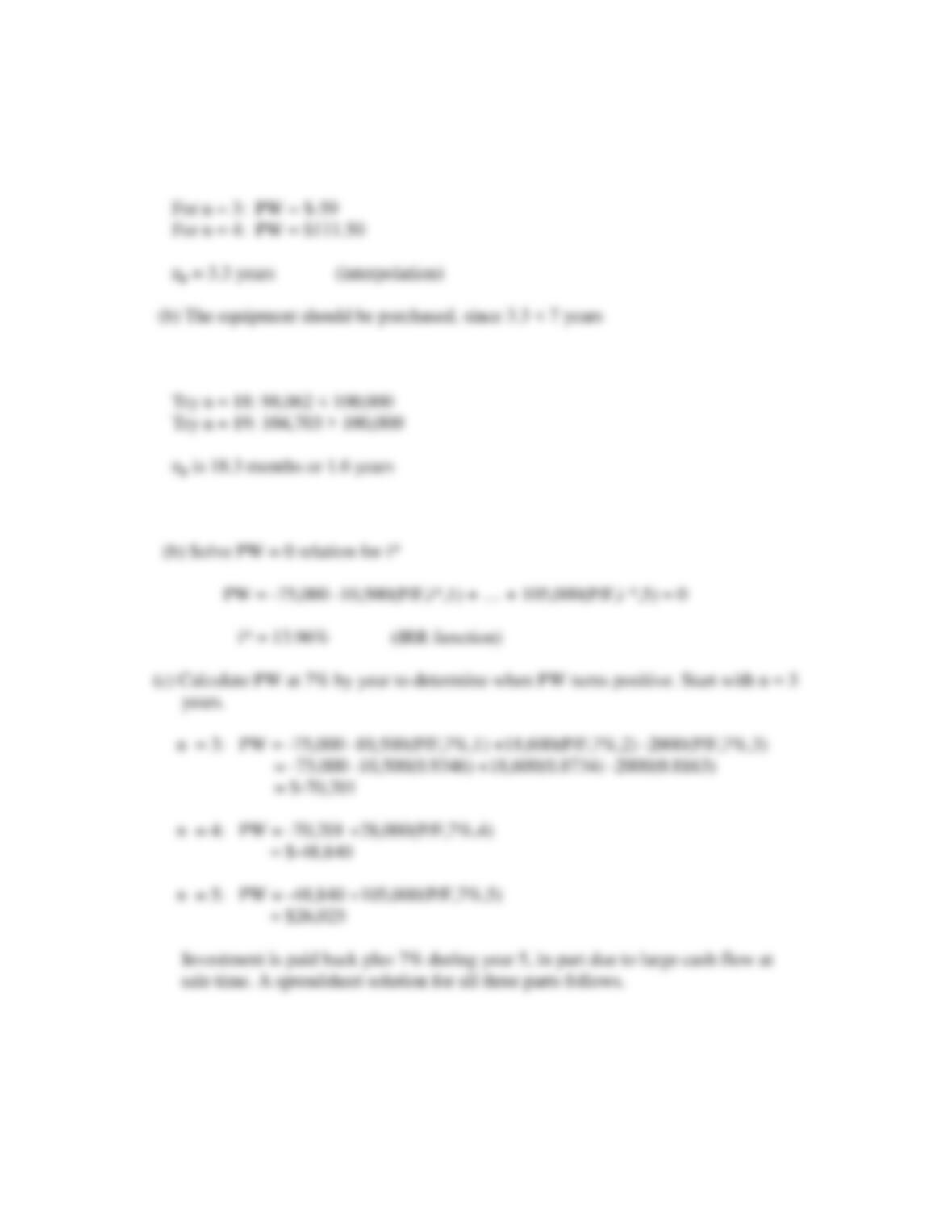
(c) Spreadsheet shows nonlinear increase in payback as MARR increases. Note that at
10
13.33 (a) Set PW = 0 and solve for np
0 = -1050 + 600(P/F,10%,np) + 175(P/A,10%,np) + 45(P/G,10%,np)
13.34 –250,000 – 500n + 250,000(1 + 0.02)n = 100,000
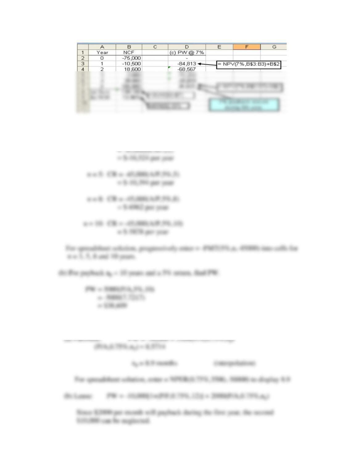
13.35 (a) Cash flows sum to $139,100, which exceeds the $75,000 first cost by 85%.
11
13.36 (a) Calculate capital return (CR) at a 5% return. S = 0.
n = 3: CR = -45,000(A/P,5%,3)
13.37 Monthly i = 9/12 = 0.75%. Solve PW relations for np
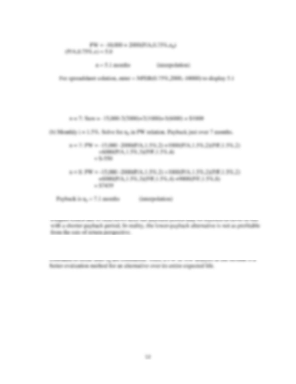
13.38 (a) Sum NCF for n months until it turns positive. Payback between 6 and 7 months.
n = 6: Sum = -15,000-2(2000)+2(1000)+2(6000) = $-5000
13.39 Since cash flows after np are neglected in payback analysis, an alternative that produces
13.40 No-return payback neglects both the time value of money and all cash flows after the 0%
payback period. Alternatives that don’t payback at 0% may be acceptable if the cash flows
13
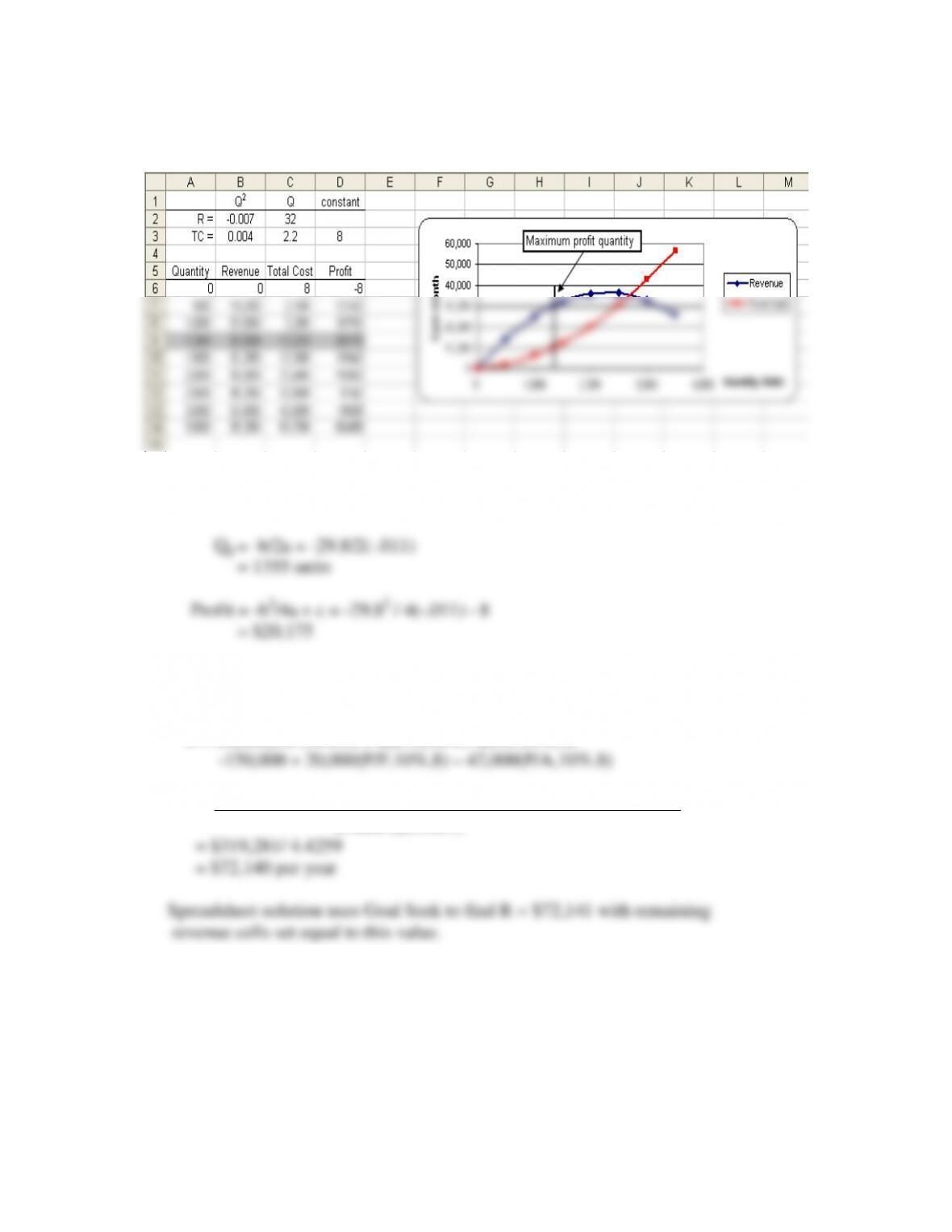
13.41 (a) Plot shows maximum quantity at about 1350 units. Profit estimate is $20,175
(b) Profit = R – TC = (-.007-.004) Q2 + (32-2.2)Q – 8
= -.011Q2 + 29.8Q – 8
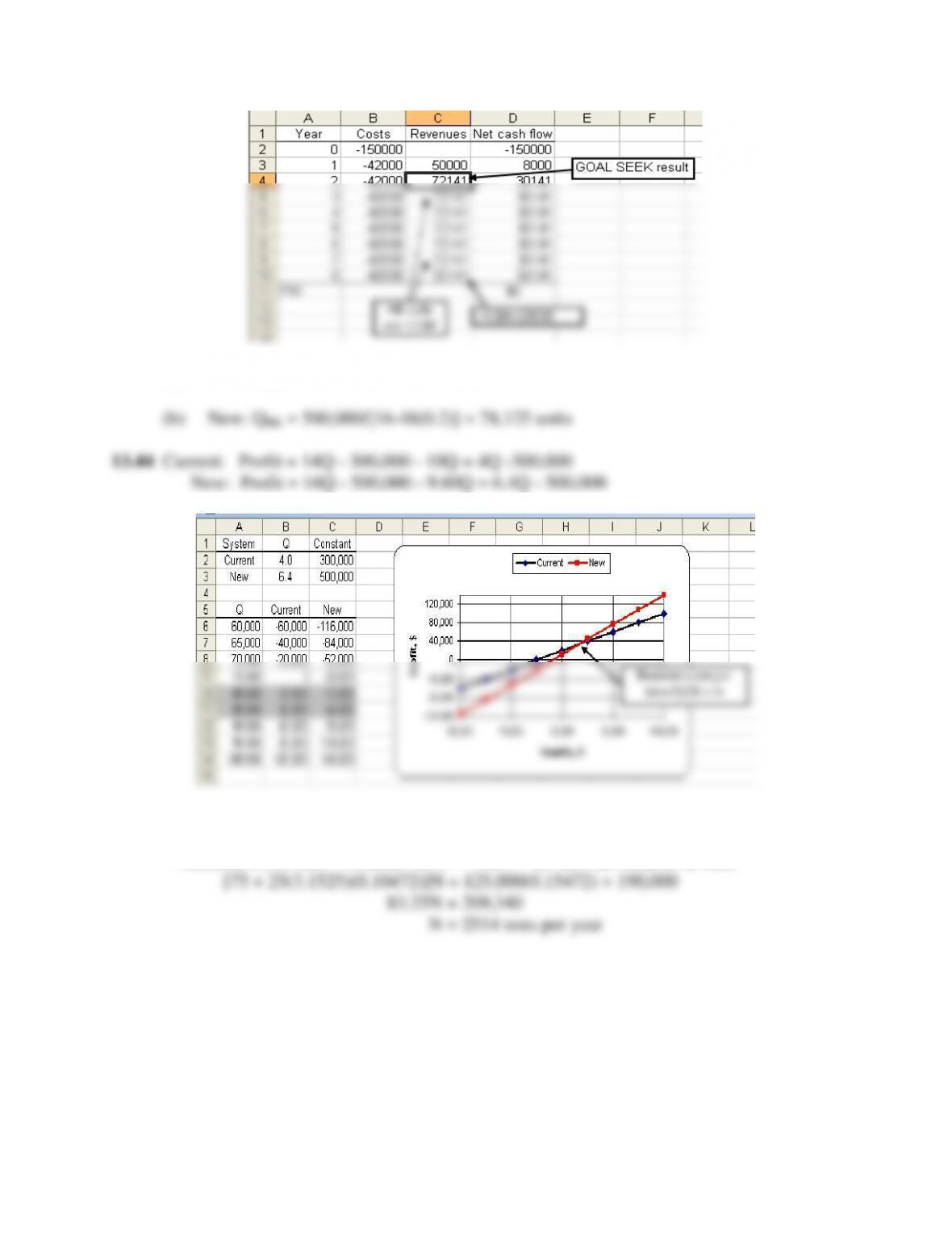
13.42 Let R = revenue for years 2 through 8. Set up PW = 0 relation.
PW = Revenue – costs
0 = 50,000(P/F,10%,1) + R(P/A,10%,7)(P/F,10%,1)
R = -50,000(0.9091) + 150,000 – 20,000(0.4665) + 42,000(5.3349)
(4.8684)(0.9091)
14
13.43 (a) Current: QBE = 300,000/(14-10) = 75,000 units
13.45 Solve the relation AWI = AWO for N = number of tests per year
-125,000(A/P,5%,8) – 190,000 -25N = -100N – 25N(F/A,5%,3)(A/F,5%,8)
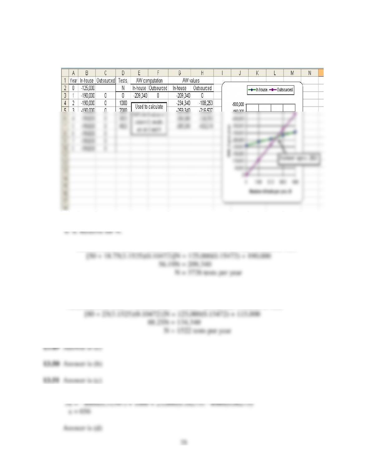
13.46 Spreadsheet used to calculate AW values for each N value; recorded in columns G
and H using ‘Paste Values’ function and then plotted.
13.47 It will raise the breakeven point. Outsourcing will cost $75, increasing to $93.75 in years
-125,000(A/P,5%,8) – 190,000 -25N = –75N – 18.75N(F/A,5%,3)(A/F,5%,8)
13.48 It will decrease the breakeven point. Resolve for N.
-125,000(A/P,5%,8) – 115,000 -20N = -100N – 25N(F/A,5%,3)(A/F,5%,8)
13.52 -23,000(A/P,10%,10) + 4000(A/F,10%,10) – 3000 – 3x = -8,000(A/P,10%,4) – 2000 – 6x
16
13.53 -100N = -250,000(A/P,15%,4) – 80,000 – 40N
13.54 -10,000 – 50x = -21,500 – 10x
13.56 -100,000(A/P,6%,10) -10,000 = -30,000(A/P,6%,5) – x
13.59 Set AW relations equal and solve for x, the cost of the enamel coating
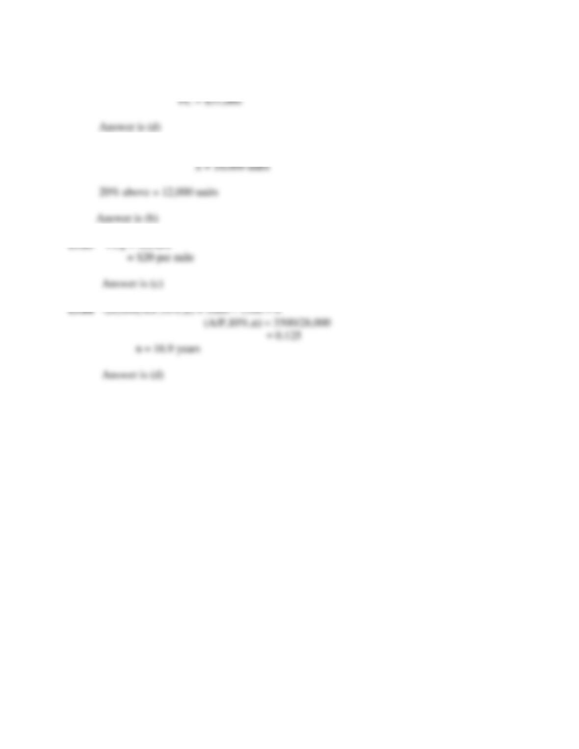
13.60 50,000 + 2400np = 25,000(F/P,20%,np)
17
13.61 -16,000 – 40(1000) = –FC – (125/5)(1000)
13.62 Breakeven: -500,000 = (250 – 200)x
18
Solution to Case Study, Chapter 13
Sometimes, there is not a definitive answer to a case study exercise. Here are example responses.
WATER TREATMENT PLANT PROCESS COSTS
1. Savings = 40 hp * 0.75 kw/hp * 0.12 $/kwh * 24 hr/day * 30.5 days/mo ÷ 0.90
2. A decrease in the efficiency of the aerator motor renders the selected alternative of “sludge
3. If the cost of lime increased by 50%, the lime costs for “sludge recirculation only” and
4. If the efficiency of the sludge recirculation pump decreased from 90% to 70%, the net savings
5. If hardness removal were discontinued, the extra cost for its removal (column 4 in Table 13-
1) would be zero for all alternatives. The favored alternative under this scenario would be
6. If the cost of electricity decreased to 8¢/kwh, the aeration only and sludge recirculation only
7. (a) For alternatives 1 and 2 to breakeven, the total savings would have to be equal to
the total extra cost of $1,849. Thus,
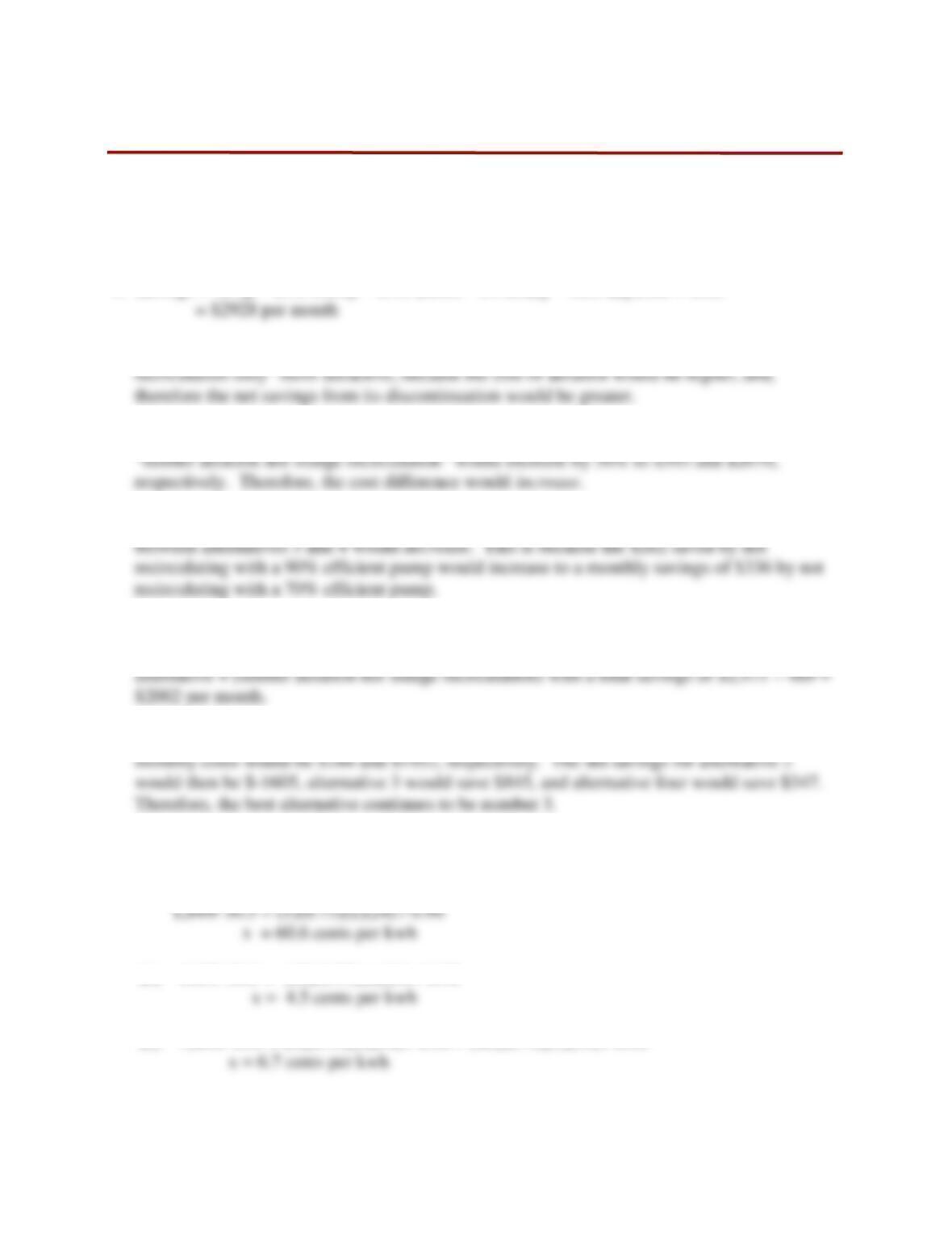
(c) 1,849/ 30.5 = (5)(0.75)(x)(24) / 0.90 + (40)(0.75)(x)(24) / 0.90