20
YZ2
YZ2
YZ2
Y2Z3
Y2Z3
Y2Z2
Y2Z2
Z
1
YZ
YZ
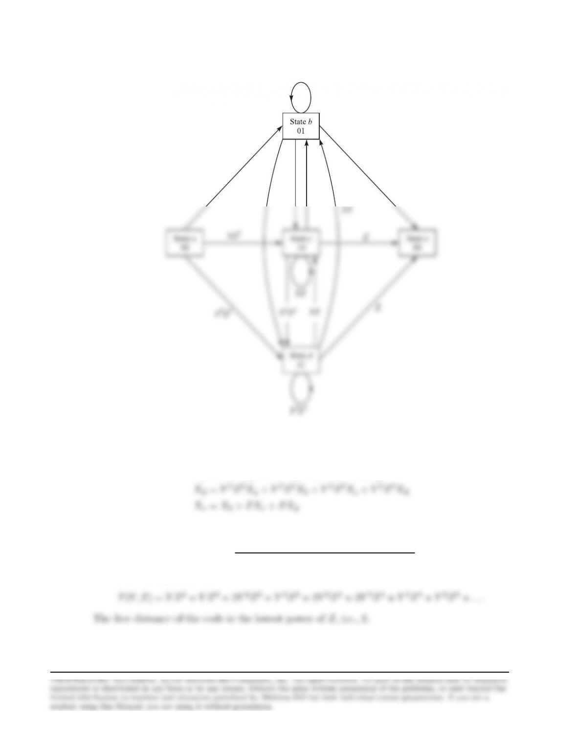
and we have the following equations
Xb=Y Z2Xa+Y Z2Xb+Y ZXc+Y ZX2
Xc=Y Z2Xa+Y Z2Xb+Y ZXc+Y ZXd
from which, after eliminating, we obtain
T(Y, Z) = Y Z2+Y Z3+Y2Z3+Y3Z3−Y3Z5
1−Y Z −Y Z2−Y2Z3−Y3Z3+Y3Z5
which can be expanded as
3. There is only one path at free distance 2, this corresponds to the input sequence 0100, with
output 011000.
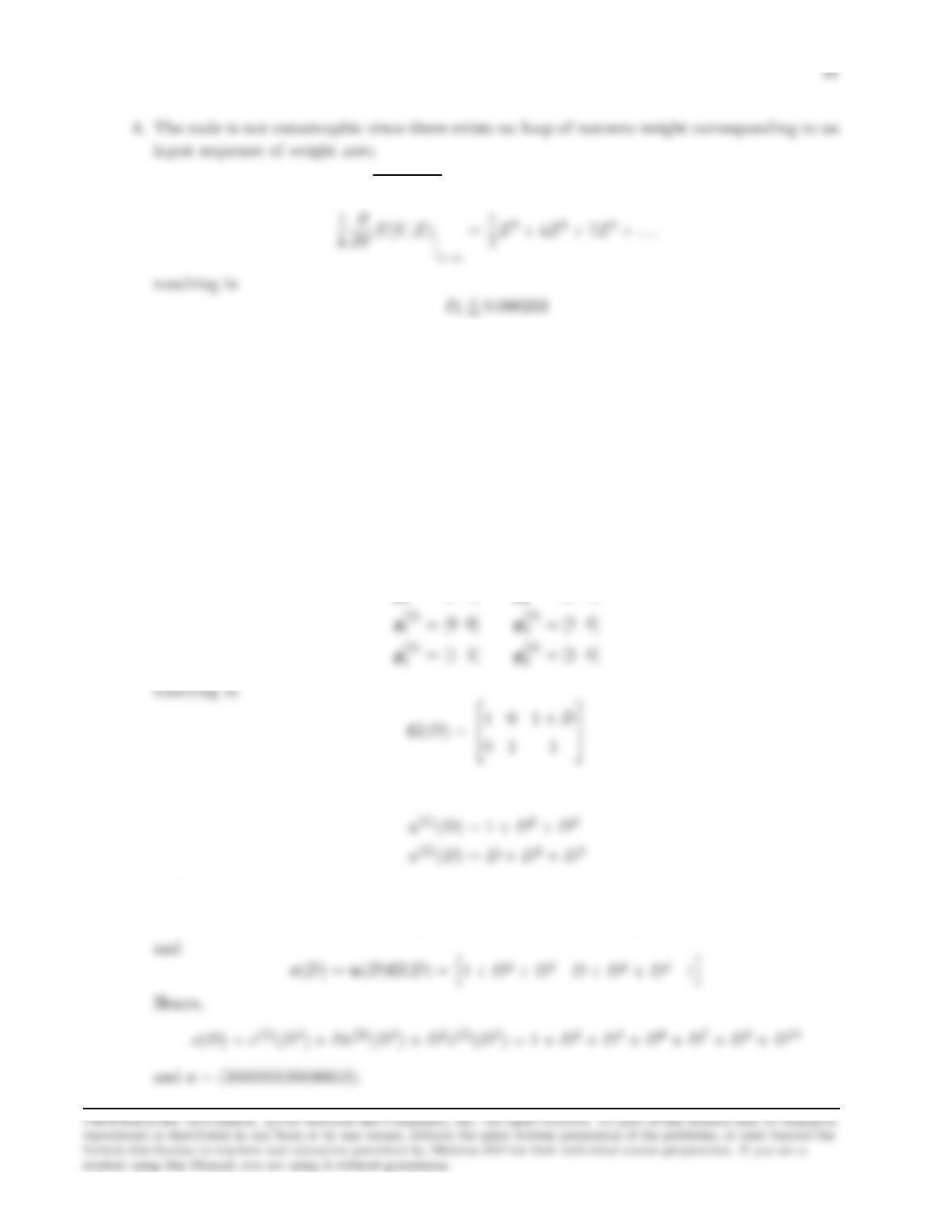
5. For p= 10−4we have ∆ = p4p(1 −p)≈0.02, and
Problem 8.13
1. For this code we have
g1= [1 0 0 0] g2= [0 1 0 0] g3= [1 1 1 0]
Therefore,
g(1)
0 1 1
2. From uwe have u(1) = (10110) and u(2) = (01101), hence
and
u(D) = h1 + D2+D3D+D2+D4i
4. We need to use Equation 8.1-38, to obtain
Problem 8.14
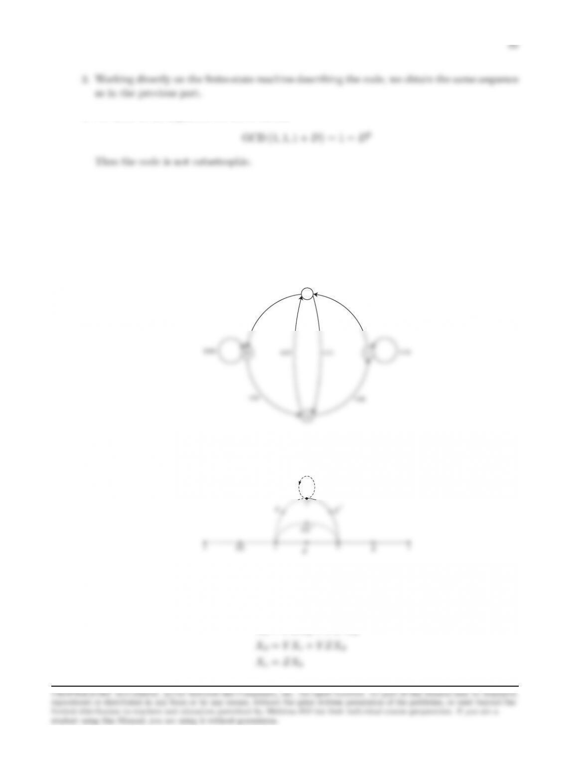
1. The state transition diagram is shown below
01
10
0/11
0/10
and the state diagram is
YZ
Y
Z
Z
Z 2
YZ
Solving the following equations
Xb=ZXc+Z2Xd
Xc=Y ZXa+Y Z2Xb
23
results in
T(Y, Z) = Xe
Xa
=Y Z3
1−Y Z −Y Z3
4. The crossover probability of the BSC is given by p=Q(√2Rcγb) where Rc=1
∂
Problem 8.15
(a)
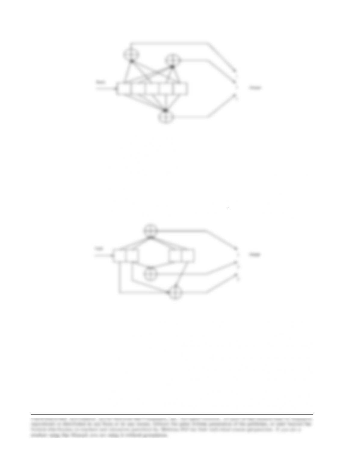
g1= [23] = [10011], g2= [35] = [11101]
(b)
g1= [25] = [10101], g2= [33] = [11011], g3= [37] = [11111]
24
Input
Output
3
2
1
(c)
g1= [17] = [1111], g2= [06] = [0110], g3= [15] = [1101]
Problem 8.16
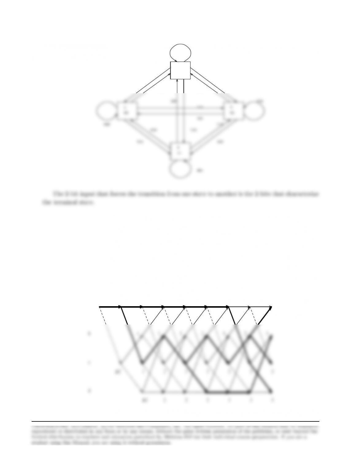
For the encoder of Probl. 8.15(c), the state diagram is as follows :
25
10
c
101
110
000
001
011
Problem 8.17
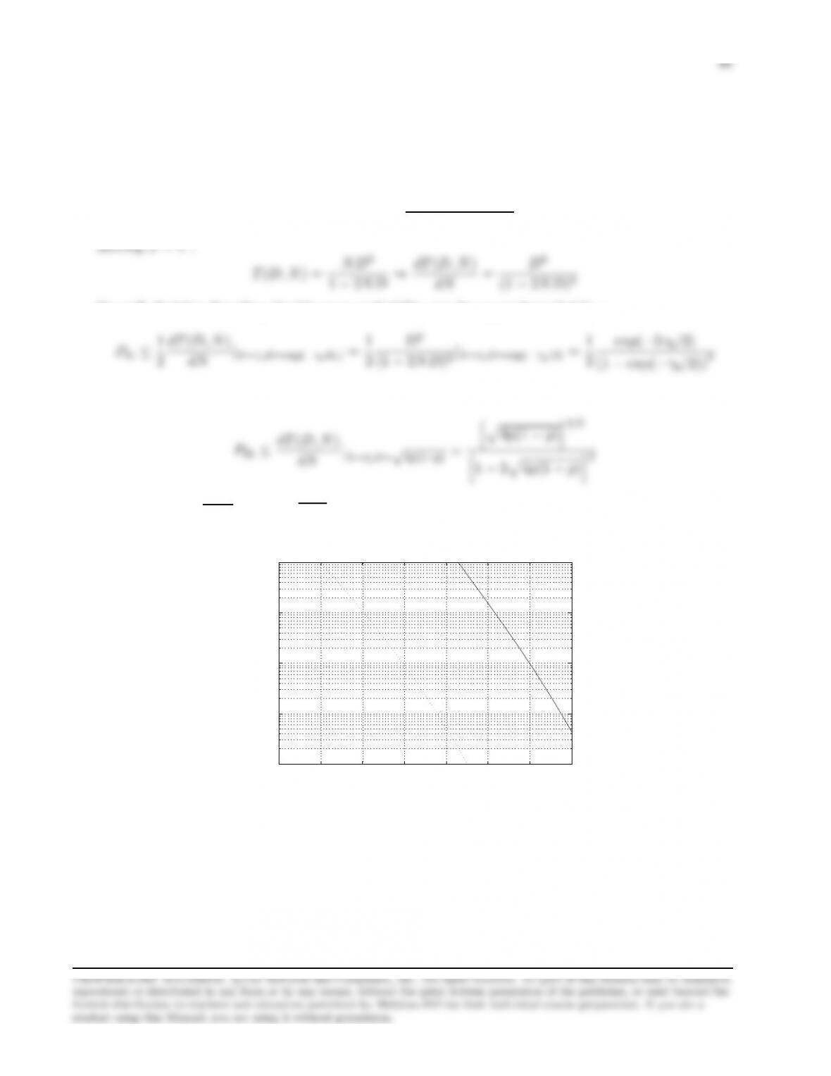
The encoder is shown in Probl. 8.8. The channel is binary symmetric and the metric for Viterbi
decoding is the Hamming distance. The trellis and the surviving paths are illustrated in the
following figure :
State
a
d=0 1 2 2 2
2 3 3
Problem 8.18
In Probl. 8.8 we found :
T(D, N, J) = J3ND5
1−JN D(1 + J)
For soft-decision decoding the bit-error probability can be upper-bounded by :
dT (D, N )
D5
exp(−5γb/2)
For hard-decision decoding, the Chernoff bound is :
dN |N=1,D=√4p(1−p)=hp4p(1 −p)i5/2
where p=Q√γbRc=Qpγb/2(assuming binary PSK). A comparative plot of the bit-error
probabilities is given in the following figure :
3 4 5 6 7 8 9 10
10−6
10−5
10−4
10−3
10−2
SNR/bit (dB)
Bit−error probability
Soft−dec. decoding
Hard−dec. decoding
Problem 8.19
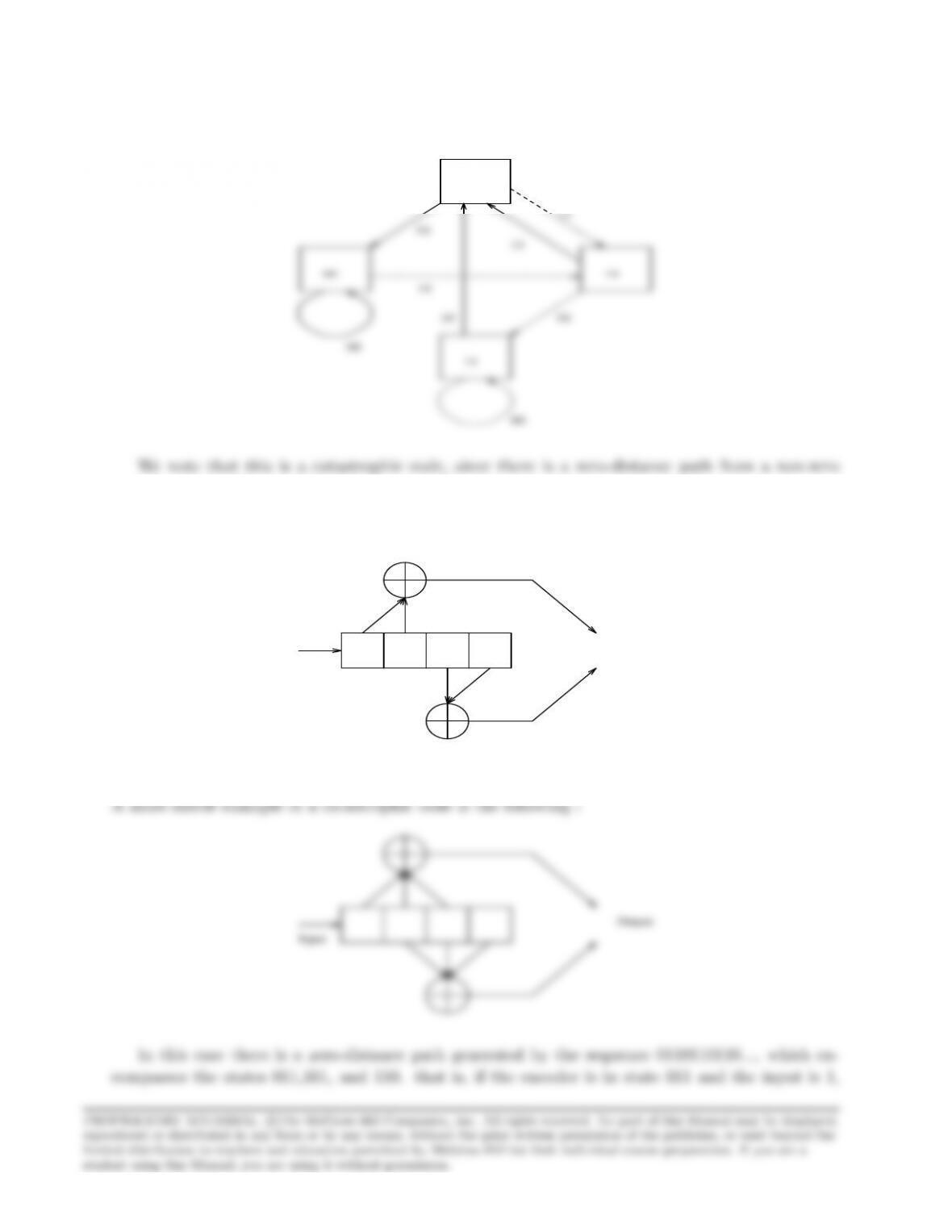
g1= [110], g2= [011],states : (a) = [00],(b) = [01],(c) = [10],(d) = [11]
27
The state diagram is given in the following figure :
01
11
11
10
10
01
00
01
state back to itself, and this path corresponds to input 1.
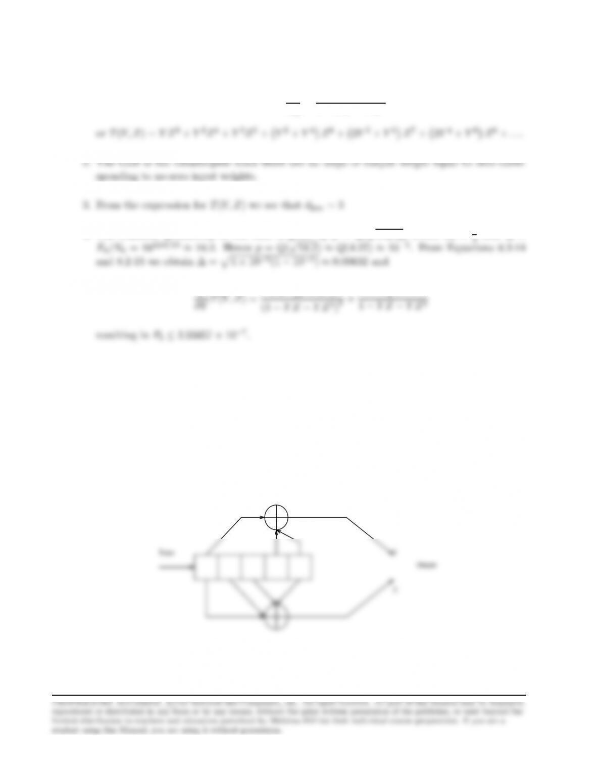
A simple example of an K= 4,rate 1/2 encoder that exhibits error propagation is the following
:
Input
Output
The state diagram for this code has a self-loop in the state 111 with input 1, and output 00.
Problem 8.20
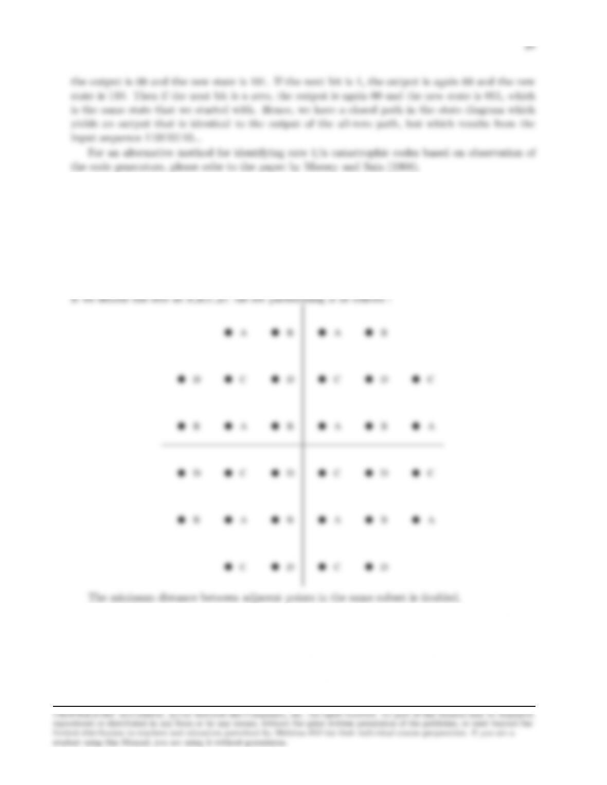
There are 4 subsets corresponding to the four possible outputs from the rate 1/2 convolutional
encoder. Each subset has eight signal points, one for each of the 3-tuples from the uncoded bits.
Problem 8.21
29
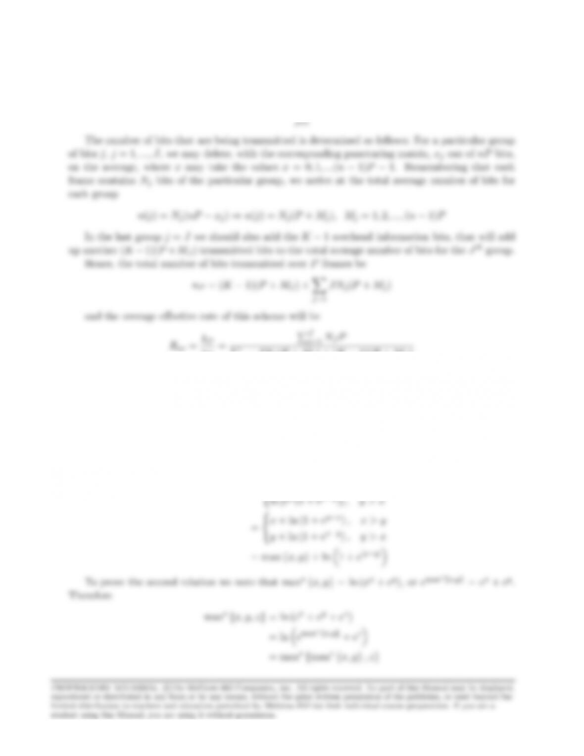
Over Pframes, the number of information bits that are being encoded is
kP=P
J
X
NJ
nP
Problem 8.22
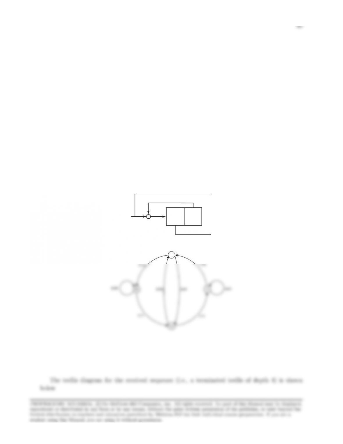
By definition, from Equation 8.8-26, we have
max∗{x, y}= ln (ex+yy)
=(ln [ex(1 + ey−x)] , x > y
Problem 8.23
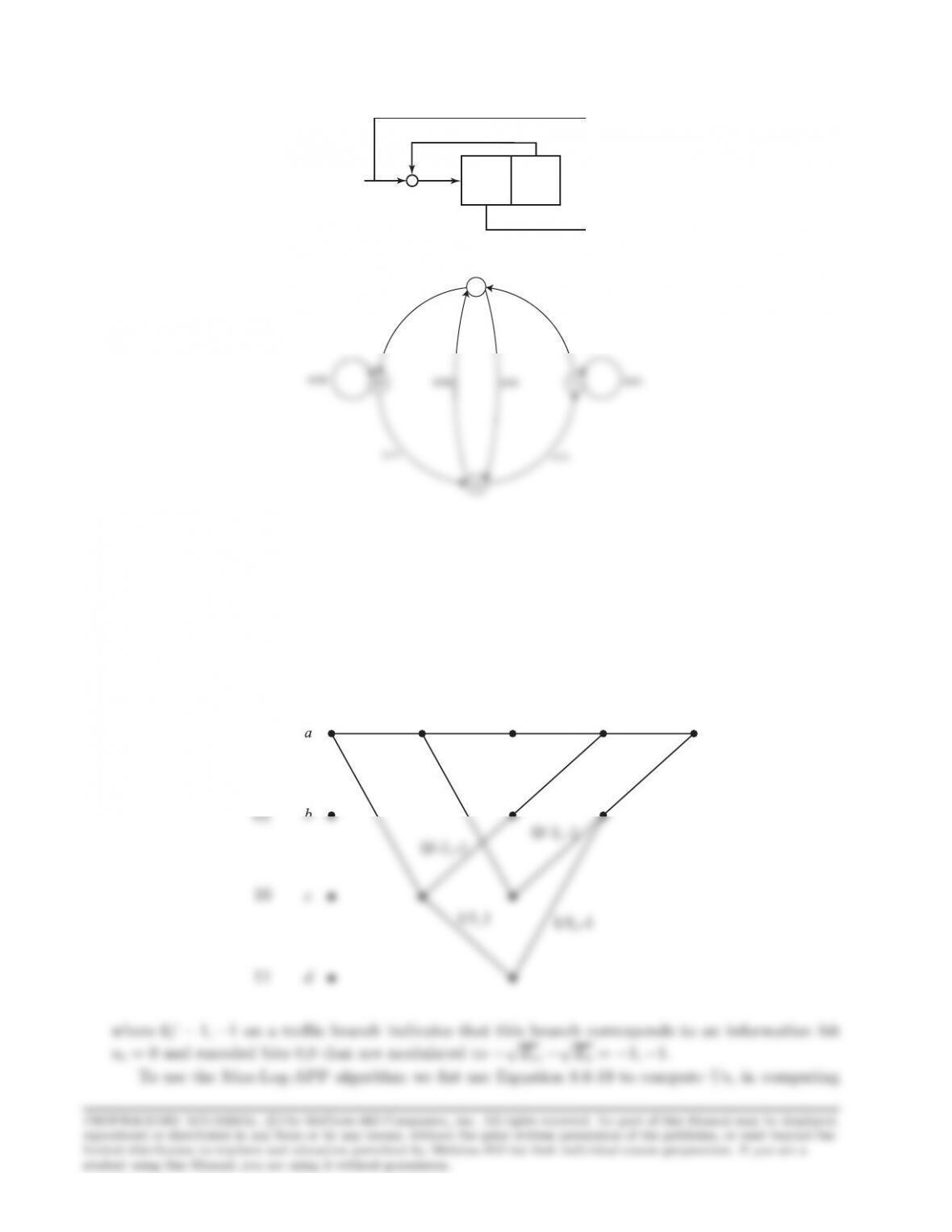
The encoder and the state transition diagram are shown below
+
01
1/10
1/10
0/-1,-1
0/-1,-1 0/-1,-1 0/-1,-1
1/1,1 1/1,1 1/1,-1 1/1,-1
(0.3,0.2) (1,-1.2) (1.2,1.7) (0.3,-0.6)
00
1. To use the BCJR algorithm we fist use Equation 8.8-20 to compute γ’s, then use the recursive
relations 8.8-11 and 8.8-14 to compute α’s and β’s and finally use Equation 8.8-17 to find the
4)
γ1(1,1) = 0.0181939 α1(1) = 0.0181939 β3(1) = 0.0250553
γ1(1,3) = 0.0299966 α1(3) = 0.0299966 β3(2) = 0.0338211
γ2(1,1) = 0.0144918 α2(1) = 0.000263662 β2(1) = 0.0000480464
32
Using these values in Equation 8.8-17, we obtain
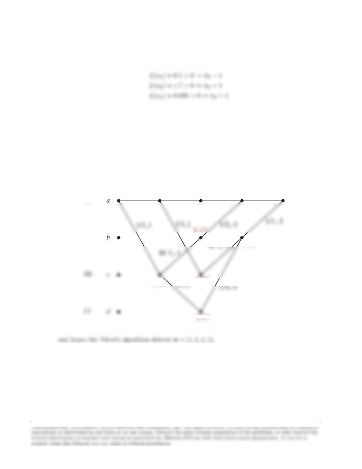
L(u1)≈1.7>0⇒ˆu1= 1
2. For Viterbi algorithm we have to minimize the Euclidean distance, the trellis with accumu-
lated metrics (in red) is shown below
0/-1,-1
0/-1,-1 0/-1,-1 0/-1,-1
(0.3,0.2) (1,-1.2) (1.2,1.7) (0.3,-0.6)
00
3.13
7.17
12.5
#
#
13.95
Problem 8.24
The encoder and the state transition diagram are shown below
33
+
01
10
1/10
1/10
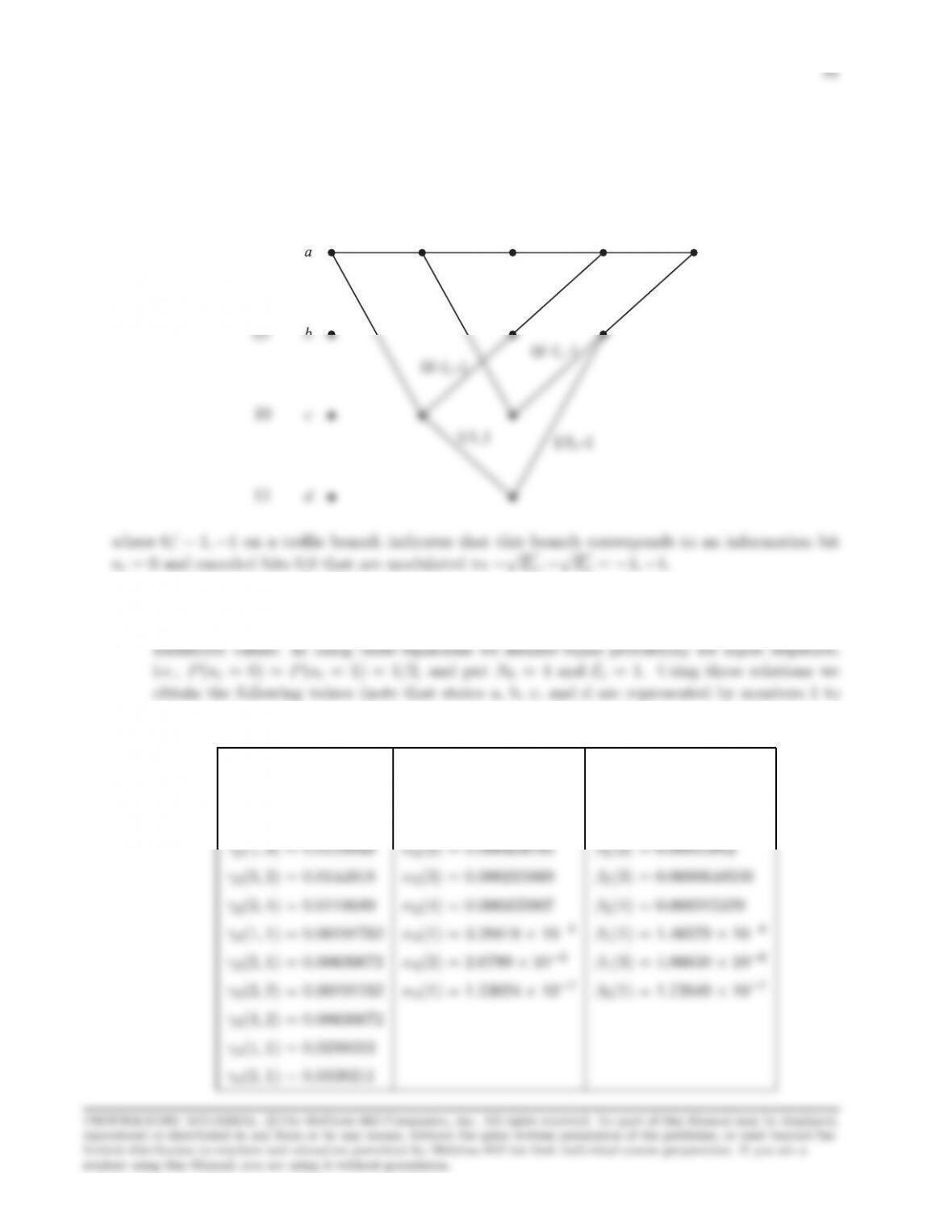
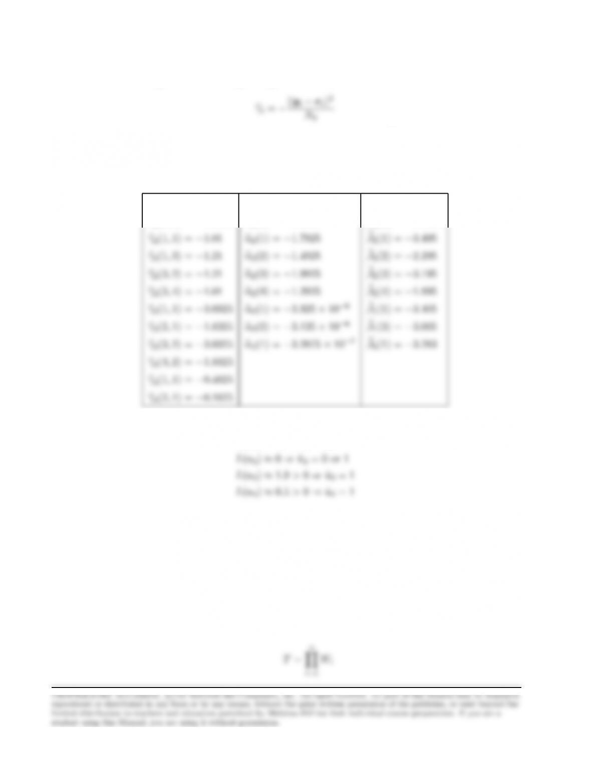
The trellis diagram for the received sequence (i.e., a terminated trellis of depth 4) is shown
below
0/-1,-1
0/-1,-1 0/-1,-1 0/-1,-1
1/1,1 1/1,1 1/1,-1 1/1,-1
(0.3,0.2) (1,-1.2) (1.2,1.7) (0.3,-0.6)
00
34
these values we drop the term corresponding to the constant coefficient and define
We then use the recursive relations in 8.8-27 to compute eα’s and e
β’s and finally use Equation
8.8-28 to find the likelihood values. In using these equations we assume equal probability for input
sequence, i.e., P(ui= 0) = P(ui= 1) = 1/2, and put N0= 4 and Ec= 1. Using these relations we
obtain the following values (note that states a, b, c, and d are represented by numbers 1 to 4)
eγ1(1,1) = −0.7825 eα1(1) = −0.7825 e
β3(1) = −0.4625
eγ1(1,3) = −0.2825 eα1(3) = −0.2825 e
β3(2) = −0.1625
Using these values in Equation 8.8-17, we obtain
L(u1)≈0.9>0⇒ˆu1= 1
Problem 8.25
1. Let us define new random variables Wi= 1 −2Xi, obviously Wi’s are independent and each
Witakes values of +1 and −1 with probabilities p(0) and p(1), respectively. This means that
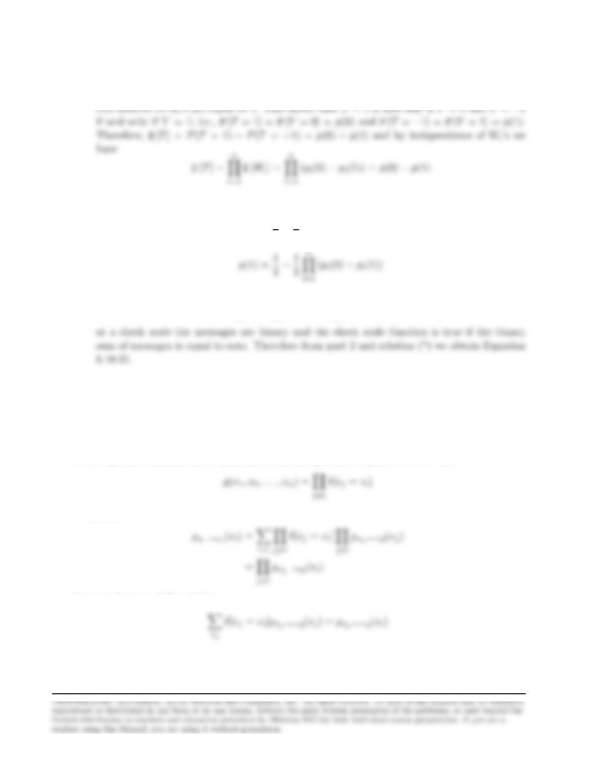
E[Wi] = pi(0) −pi(1). We also define
n
Y
35
Tis equal to +1 or −1 if an even or odd number of Wi’s are equal to −1, or equivalently if
an even or odd number of Xi’s are equal to 1. Similarly Yis equal to 0 or 1 if an even or
i=1
i=1
2. From part 1 and p(0) + p(1) = 1 we obtain
p(0) = 1
2+1
2
n
Y
i=1
(pi(0) −pi(1))
2−1
2
n
Y
i=1
3. Note that
pj(0) −pj(1) = 1 −2pj(1) (∗)
Problem 8.26
For an equality constraint node (cloning node) that generates replicas of xiwe have
j6=i
Using Equation 8.10-22 we have
j6=i
where we have used the relation
Problem 8.27
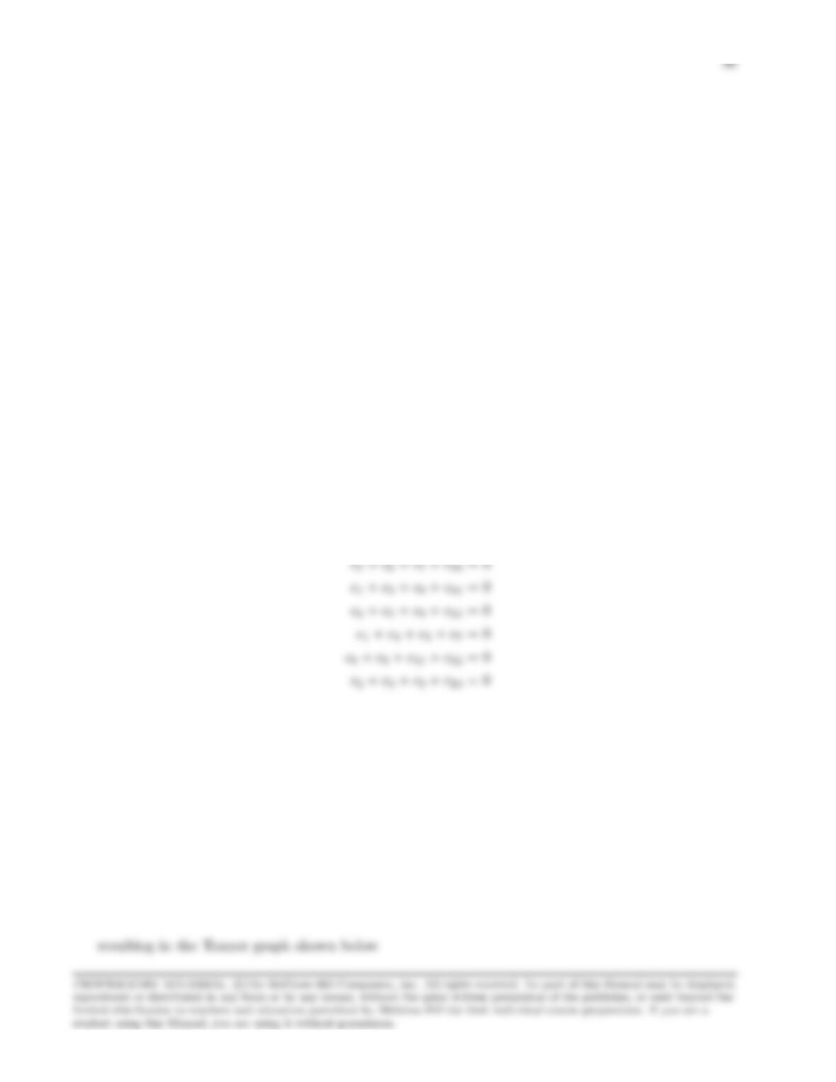
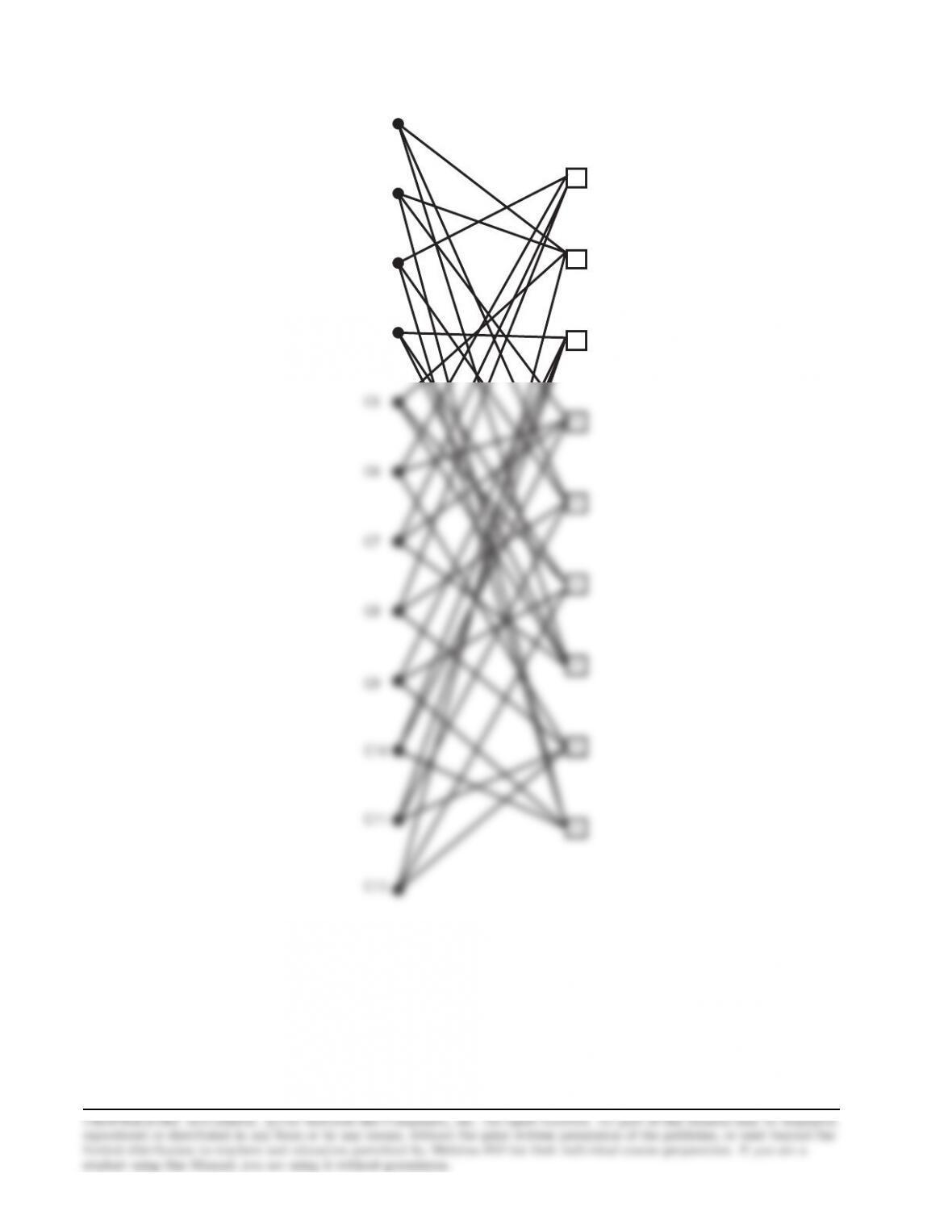
From Hwe have the following parity check equations
c3+c6+c7+c8= 0
c1+c2+c5+c12 = 0
c4+c9+c10 +c11 = 0
37
+
+
+
C1
C2
C3
C4
Problem 8.28
38
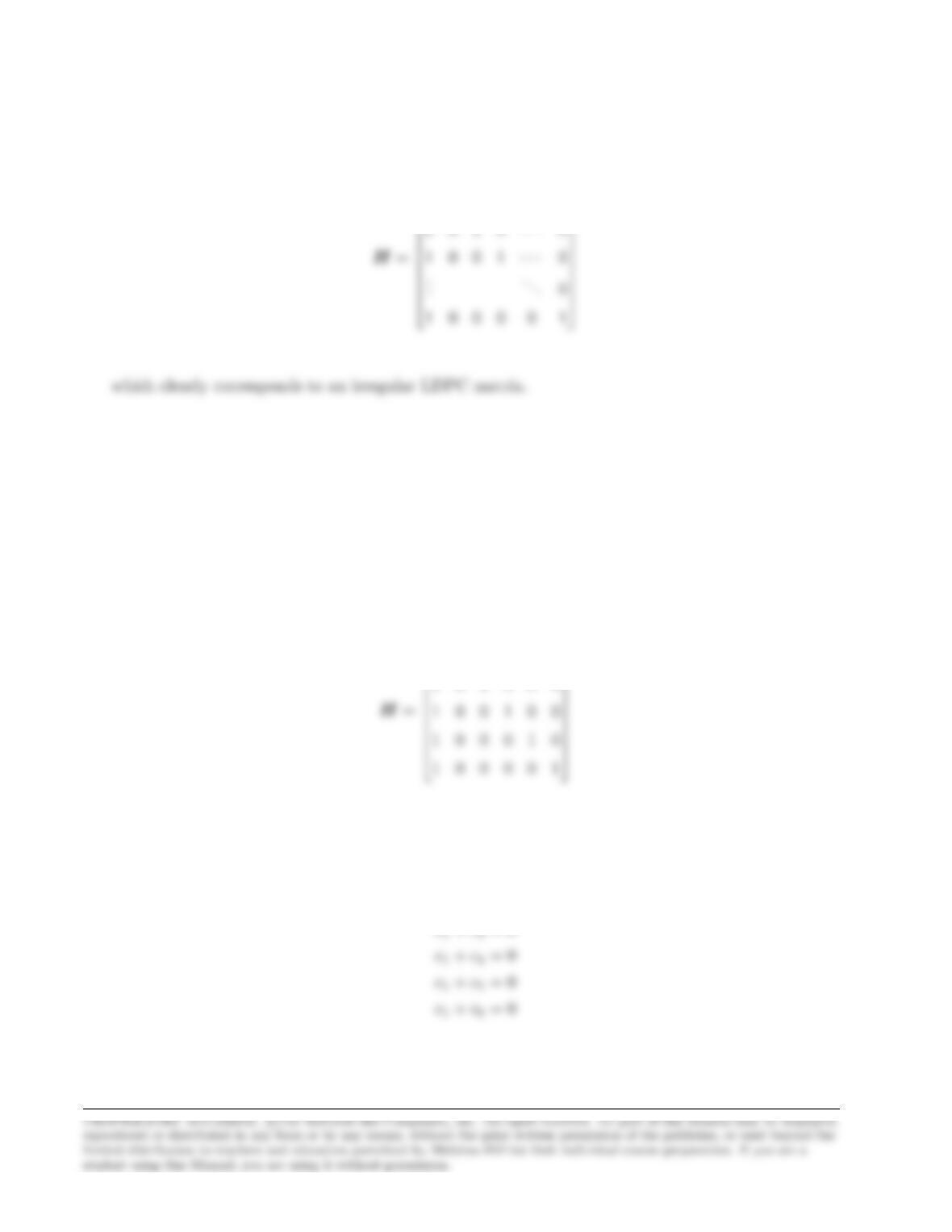
For a repetition code G= [1 1 1 … 1] and hence
1 1 0 0 ··· 0
1 0 1 0 ··· 0
Problem 8.29
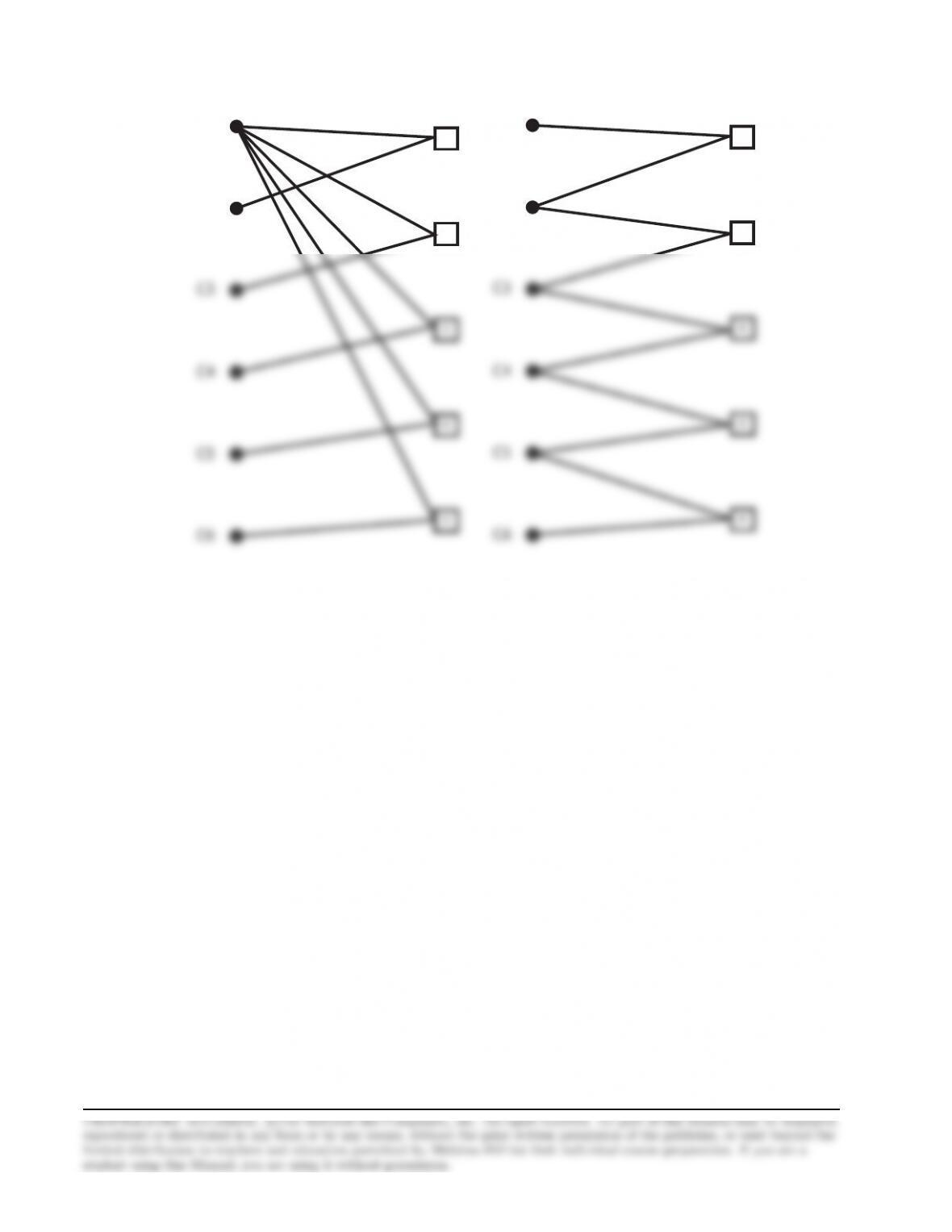
We have
1 1 0 0 0 0
and the parity check equations are
c1+c2= 0
c1+c3= 0
Two Tanner graphs for this code are shown below
39
+
+
C1
C2
+
+
C1
C2