978-0072957167 Chapter 6 Part 1

Solutions Manual

for

Digital Communications, 5th Edition

(Chapter 6) 1

Prepared by

Kostas Stamatiou

January 11, 2008

2

Problem 6.1

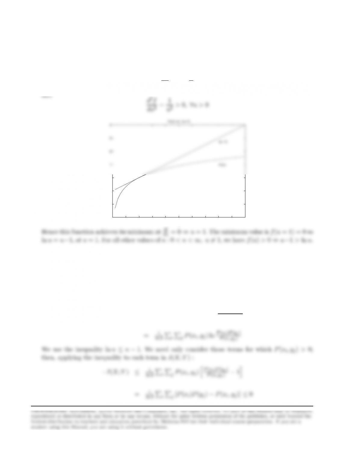
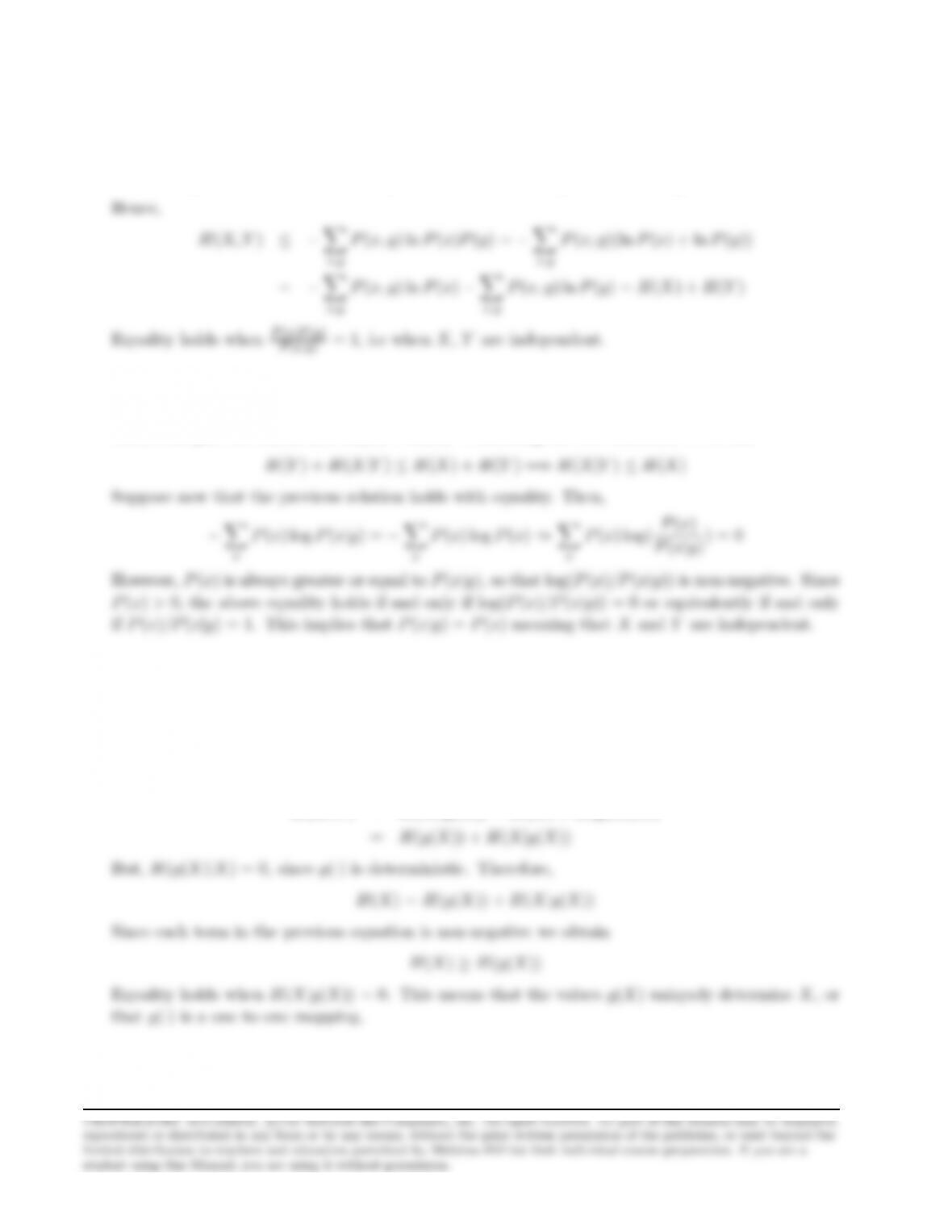
Let f(u) = u−1−ln u. The first and second derivatives of f(u) are

df

du = 1 −1

u

0 0.5 1 1.5 2 2.5 3 3.5 4 4.5 5

−3

−2

−1

0

1

2

3

4

u

ln(u) vs. (u−1)

(u−1)

ln(u)

Hence this function achieves its minimum at df

du = 0 ⇒u= 1.The minimum value is f(u= 1) = 0 so

ln u=u−1,at u= 1.For all other values of u: 0 < u < ∞, u 6= 1,we have f(u)>0⇒u−1>ln u.

Problem 6.2

We will show that −I(X;Y)≤0

−I(X;Y) = −PiPjP(xi, yj) log 2P(xi,yj)

P(xi)P(yj)

3

The first inequality becomes equality if and only if

when P(xi, yj)>0.Also, since the summations

iX

j

contain only the terms for which P(xi, yj)>0,this term equals zero if and only if P(Xi)P(Yj) = 0,

Problem 6.3

We shall prove that H(X)−log n≤0 :

H(X)−log n=Pn

i=1 pilog 1

pi−log n

=Pn

i=1 pilog 1

pi−Pn

i=1 pilog n

Problem 6.4

1.

H(X) = −

∞

X

k=1

p(1 −p)k−1log2(p(1 −p)k−1)

∞

X

∞

X

2. Clearly P(X=k|X > K) = 0 for k≤K. If k > K, then

But,

P(X > K) =

∞

X

k=K+1

p(1 −p)k−1=p ∞

X

k=1

(1 −p)k−1−

K

X

k=1

(1 −p)k−1!

so that

P(X=k|X > K) = p(1 −p)k−1

(1 −p)K

that is P(X=k|X > K) is the geometrically distributed. Hence, using the results of the first part

we obtain

H(X|X > K) = −

∞

X

p(1 −p)l−1log2(p(1 −p)l−1)

Problem 6.5

The marginal probabilities are given by

P(X= 0) = X

k

P(X= 0, Y =k) = P(X= 0, Y = 0) + P(X= 0, Y = 1) = 2

3

k

Hence,

H(X) = −

1

X

Pilog2Pi=−(1

3log2

1

3+1

3log2

1

3) = .9183

1

X

1

Problem 6.6

1. The marginal distribution P(x) is given by P(x) = PyP(x, y). Hence,

H(X) = −X

P(x) log P(x) = −X

P(x, y) log P(x)

2. Using the inequality ln w≤w−1 with w=P(x)P(y)

P(x,y), we obtain

6

Multiplying the previous by P(x, y) and adding over x,y, we obtain

X

x,y

P(x, y) ln P(x)P(y)−X

x,y

P(x, y) ln P(x, y)≤X

x,y

P(x)P(y)−X

x,y

P(x, y) = 0

3.

H(X, Y ) = H(X) + H(Y|X) = H(Y) + H(X|Y)

Also, from part 2., H(X, Y )≤H(X) + H(Y). Combining the two relations, we obtain

Problem 6.7

H(X, Y ) = H(X, g(X)) = H(X) + H(g(X)|X)

Problem 6.8

H(X1X2…Xn) = −

m1

X

j1=1

m2

X

j2=1

…

mn

X

jn=1

P(x1, x2, …, xn) log P(x1, x2, …, xn)

Since the {xi}are statistically independent :

P(x1, x2, …, xn) = P(x1)P(x2)…P (xn)

j2=1

jn=1

(similarly for the other xi).Then :

H(X1X2…Xn) = −Pm1

j1=1 Pm2

j2=1 … Pmn

jn=1 P(x1)P(x2)…P (xn) log P(x1)P(x2)…P (xn)

Problem 6.9

The conditional mutual information between x3and x2given x1is defined as :

I(x3;x2|x1) = log P(x3, x2|x1)

P(x3|x1)P(x2|x1)= log P(x3|x2x1)

P(x3|x1)

8

Since I(X3;X2|X1)≥0,it follows that :

Problem 6.10

Assume that a > 0.Then we know that in the linear transformation Y=aX +b:

pY(y) = 1

apX(y−b

a)

Problem 6.11

The linear transformation produces the symbols :

Problem 6.12

H= lim

n→∞ H(Xn|X1,…,Xn−1)

However, for a stationary process P(xn, xn−1) and P(xn|xn−1) are independent of n, so that

Problem 6.13

First, we need the state probabilities P(xi), i = 1,2.For stationary Markov processes, these can

be found, in general, by the solution of the system :

i

where Pis the state probability vector and Π is the transition matrix : Π[ij] = P(xj|xi).However,

in the case of a two-state Markov source, we can find P(xi) in a simpler way by noting that the

Then :

H(X) = 





P(x1) [−P(x1|x1) log P(x1|x1)−P(x2|x1) log P(x2|x1)] +

P(x2) [−P(x1|x2) log P(x1|x2)−P(x2|x2) log P(x2|x2)] 





10

If the source is a binary DMS with output letter probabilities P(x1) = 0.6, P (x2) = 0.4,its entropy

will be :

Problem 6.14

Let X= (X1, X2, …, Xn),Y= (Y1, Y2, …, Yn).Since the channel is memoryless : P(Y|X) =

Qn

i=1 P(Yi|Xi) and :

I(X;Y) = PXPYP(X,Y) log P(Y|X)

P(Y)

For statistically independent input symbols :

Pn

i=1 I(Xi;Yi) = Pn

i=1 PXiPYiP(Xi, Yi) log P(Yi|Xi)

P(Yi)

Then :

I(X;Y)−Pn

i=1 I(Xi;Yi) = PXPYP(X,Y) log QiP(Yi)

P(Y)

Problem 6.15

11

By definition, the differential entropy is

H(X) = −Z∞

−∞

p(x) log p(x)dx

Problem 6.16

The source entropy is :

5

X

i=1

pi

1. When we encode one letter at a time we require ¯

R= 3 bits/letter . Hence, the efficiency is

2. If we encode two letters at a time, we have 25 possible sequences. Hence, we need 5 bits per

3. In the case of encoding three letters at a time we have 125 possible sequences. Hence we need

Problem 6.17

Given (n1, n2, n3, n4) = (1,2,2,3) we have :

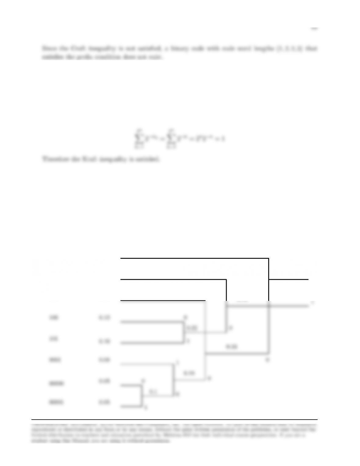
Problem 6.18

Problem 6.19

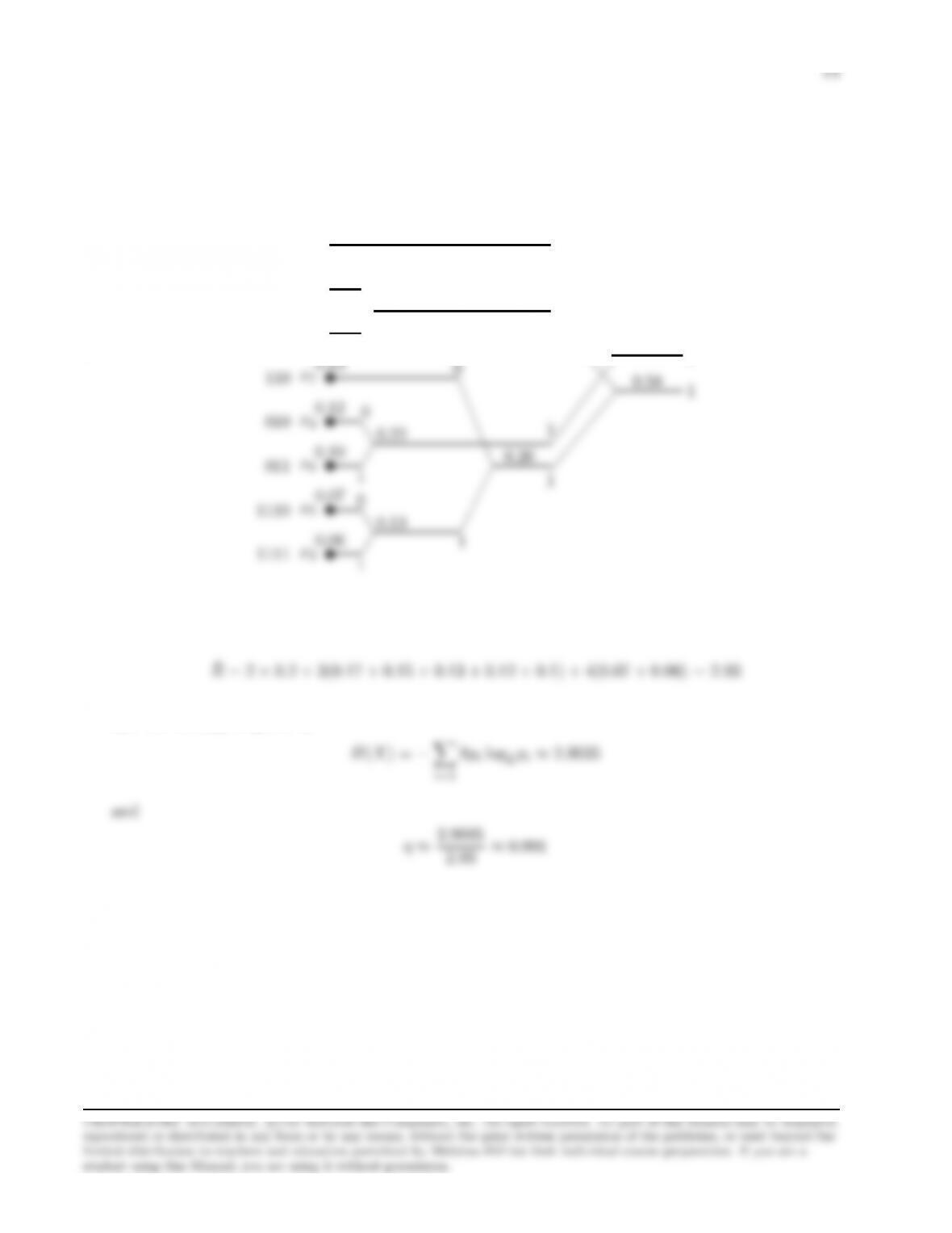
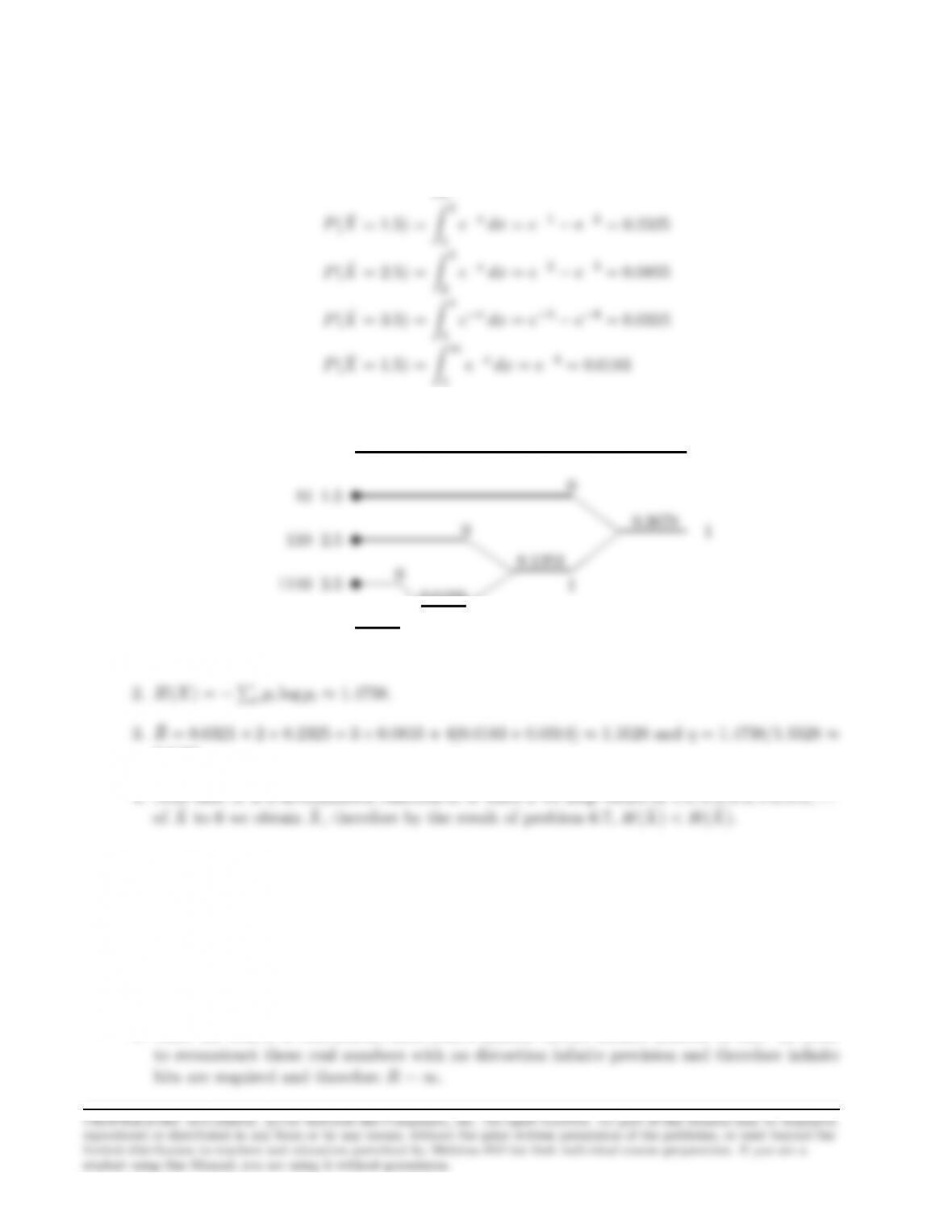
1. The following figure depicts the design of a ternary Huffman code (we follow the convention

that the lower-probability branch is assigned a 1) :

.

Codeword Probability

0.25

0.20

0.15

0.42

0.58 0

1

01

11

001

2. The average number of binary digits per source letter is :

i

3. The entropy of the source is :

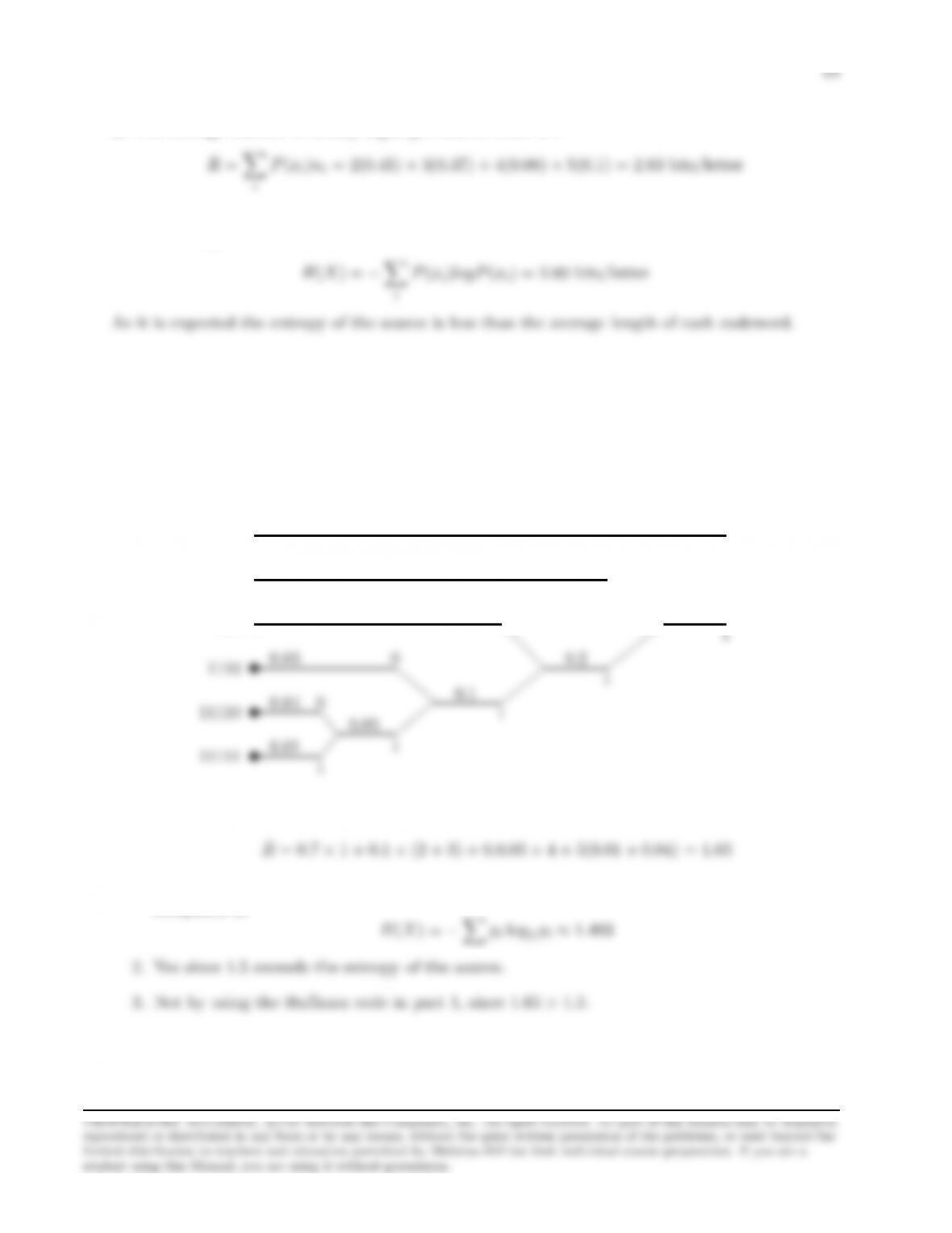
Problem 6.20

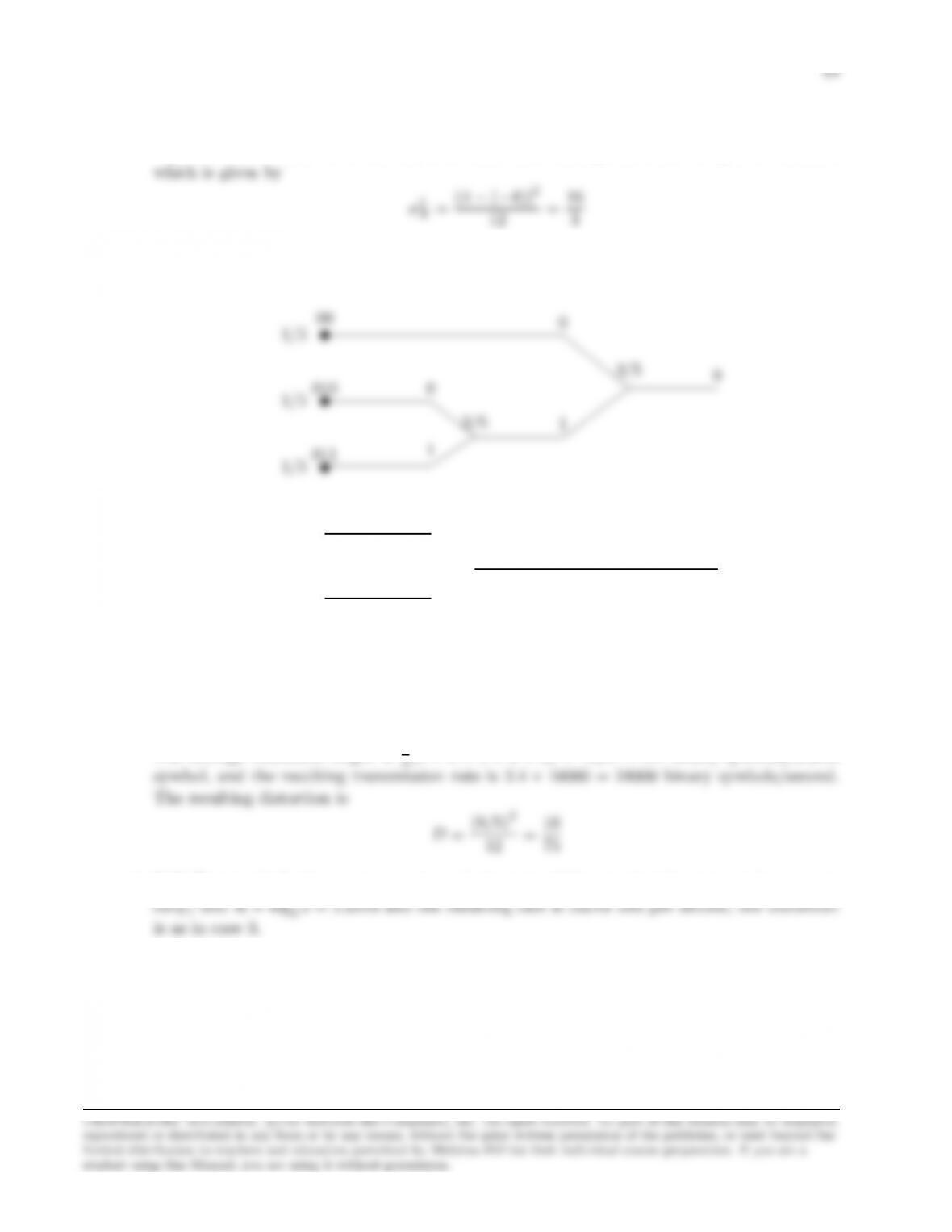
1. The Huffman tree and the corresponding code is shown below:

✉

0.1

0.12

0.15

❩❩❩

❩

★

❧❧❧

❧

✑

0.3

0

10

110

The average codeword length is given by

and the minimum possible average codeword length is equal to the entropy of the source

computed as

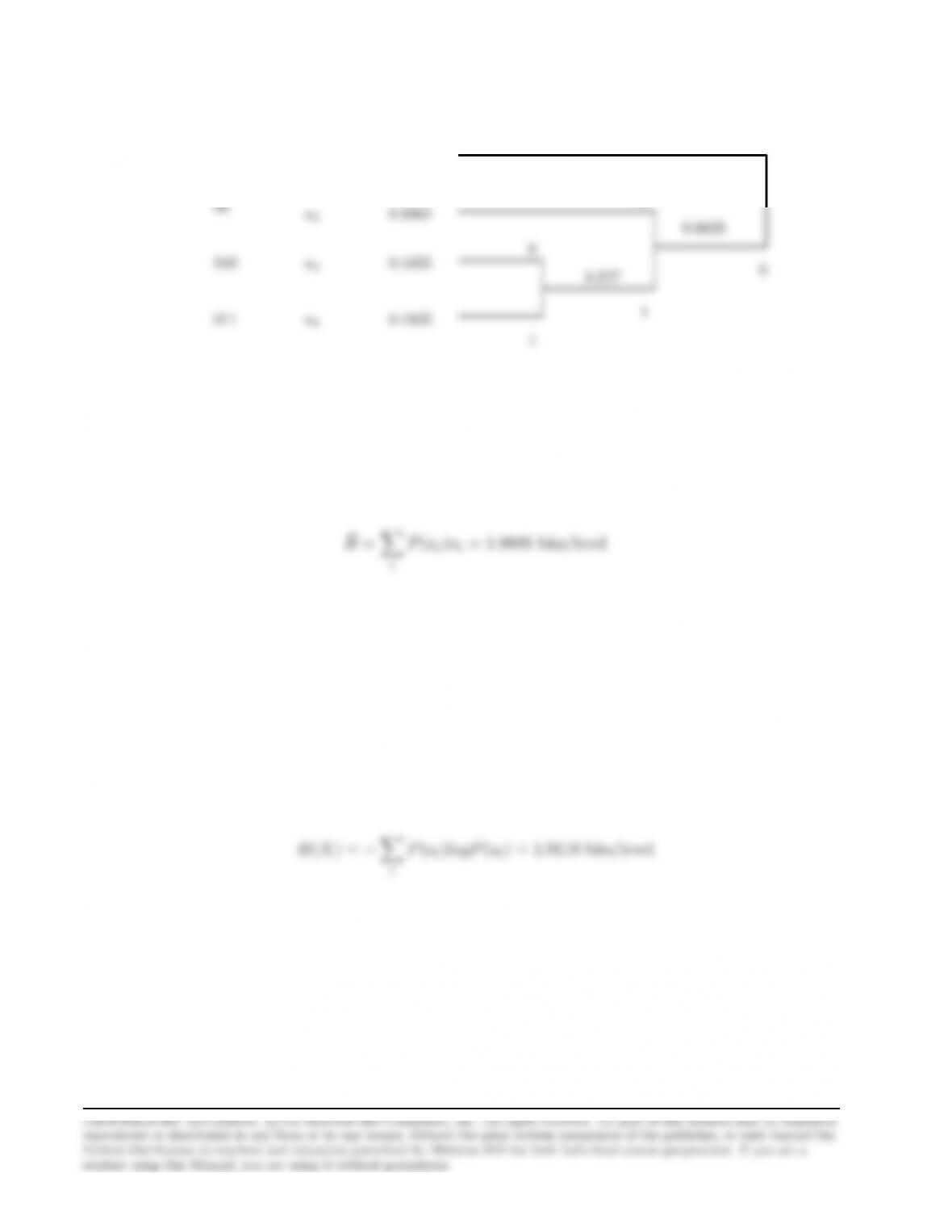
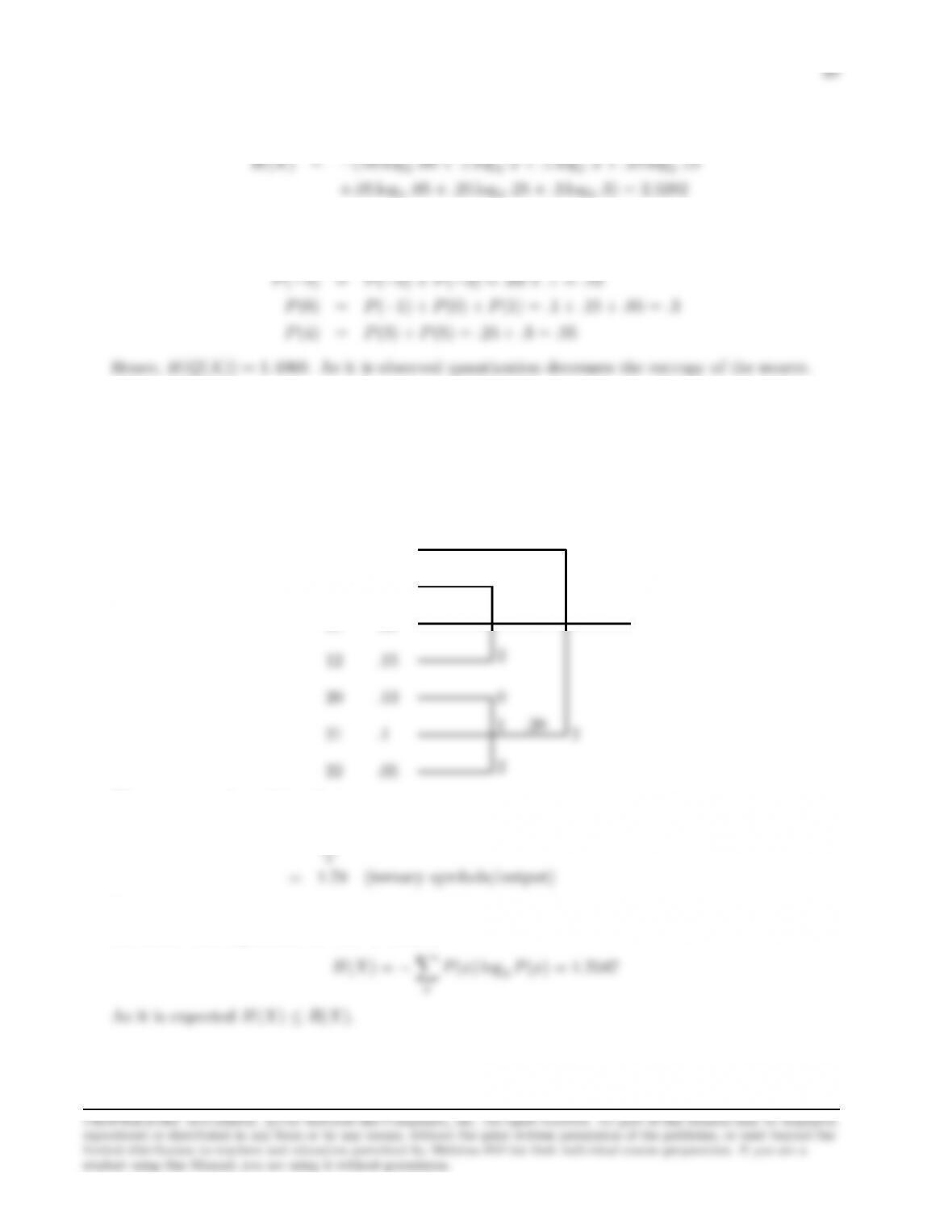
Problem 6.21

The Huffman tree is shown below

✉

x1

x8

x4

❚

✔

0.32

❚❚❚❚❚❚❚

❚

0.42

❡❡❡❡❡

0

1

00

100

101

0.20

0.17

0.15

The average codeword length is given by

and the entropy is given by

Problem 6.22

1. The following figure depicts the design of the Huffman code, when encoding a single level at a

time :

15

Codeword Level Probability

a1

0.3365

1

0

1

The average number of binary digits per source level is :

i

The entropy of the source is :

i

2. Encoding two levels at a time :

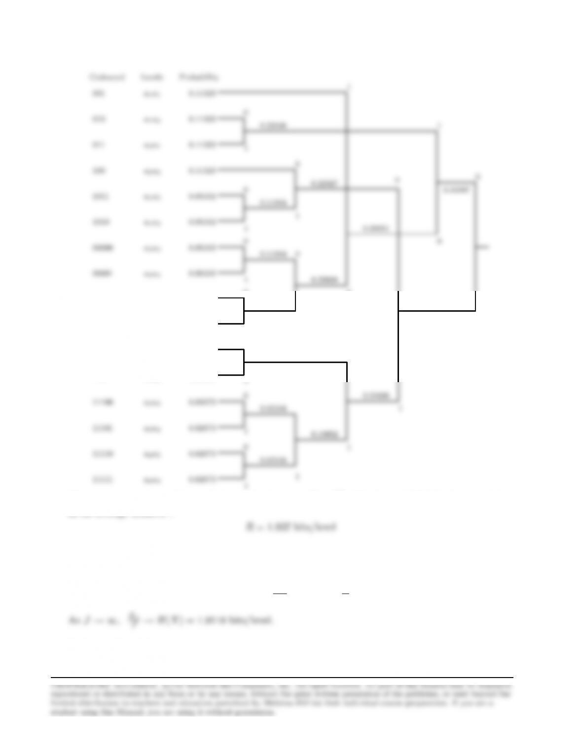
16

a3a2

a4a1

a4a2

a3a3

a3a4

a4a3

a4a4

Codeword ProbabilityLevels

a3a1

0.05502

0.02673

0

1

0.11004

0.05346

0.10692

0.22008

0.21696

0.44023

1

0

00010

00011

1100

1101

11100

11101

11110

11111

The average number of binary digits per level pair is ¯

R2=PkP(ak)nk= 3.874 bits/pair resulting

in an average number :

3.

H(X)≤¯

RJ

J< H(X) + 1

J

RJ

Problem 6.23

1. The entropy is

7

X

i=1

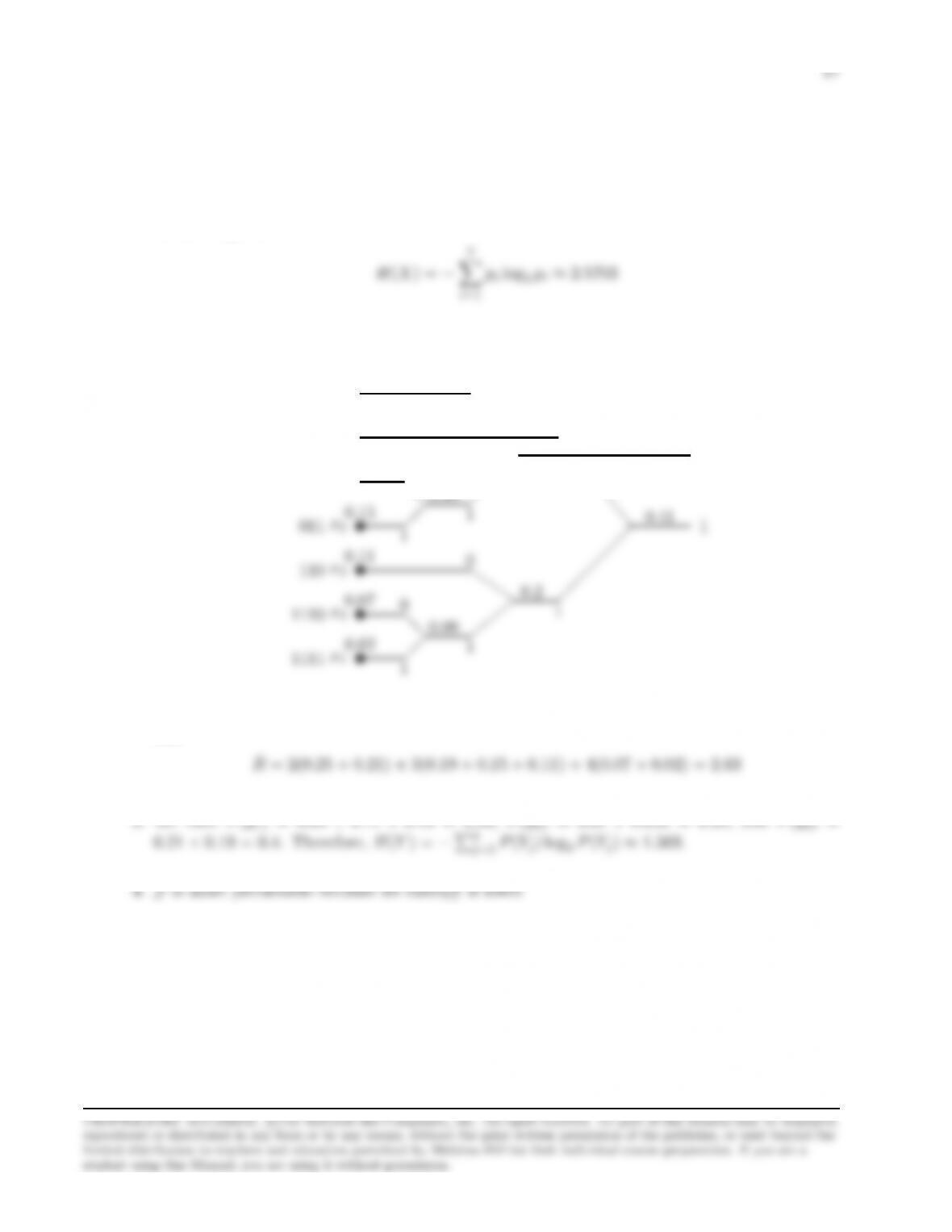
2. The Huffman tree is shown below

✉

x7

x4

x6

0.25

0.21

0.19

00

10

010

❅

❡❡❡❡❡

❙❙❙❙



0.59 0

0

and

Problem 6.24

18

1. We have

P(ˆ

X= 0.5) = Z1

0

e−xdx = 1 −e−1= 0.6321

4

and the Huffman tree is shown below

✉

0.5

6

0

1111

❅



✑

0

1

0.0498

0.9491.

4. Note that ˆ

Xis a deterministic function of ˜

Xsince if we map values of 4.5,5.5,6.5,7.5,8.5, . . .

Problem 6.25

1. Since the source is continuous, each source symbol carries infinite number of bits. In order

2. For squared error distortion, the best estimate in the absence of any side information is the

expected value which is zero in this case and the resulting distortion is equal to variance

3. An optimal uniform quantizer generates five equiprobable outputs each with probability 1/5.

The Huffman code is designed in the following diagram

✉

❝❝

❝

✑

1/5

2/5

1

0

1

10

11

The average codeword length is 1

4. If Huffman code for long sequences is used, the rate will be equal to the entropy (asymptoti-

Problem 6.26

1.

2. After quantization, the new alphabet is B={−4,0,4}and the corresponding symbol probabil-

ities are given by

Problem 6.27

The following figure depicts the design of a ternary Huffman code.

22

20

12

11

10

0

2

1

0

2

1

0

1

0

.50

.28

.05

.13

.15

.17

.18

.22

The average codeword length is

¯

R(X) = X

P(x)nx=.22 + 2(.18 + .17 + .15 + .13 + .10 + .05)

For a fair comparison of the average codeword length with the entropy of the source, we compute

the latter with logarithms in base 3. Hence,