978-0072957167 Chapter 4 Part 4

53

1. For detection of m1, we treat m2as a RV taking 1 or 2 with equal probability. The detection

rule is

arg max

s1∈{−1,1}

pn1(r1−s1−α)pn2(r2−β) + pn1(r1−s1+α)pn2(r2+β)

similarly for detection of m2we have

(s21,s22)∈{(α,β),(−α,−β)}

These relations reduce to

D+1 ⇔e

2r1

N0cosh 2αr1−2α+ 2βr2

N0> e−2r1

N0cosh 2αr1+ 2α+ 2βr2

N0

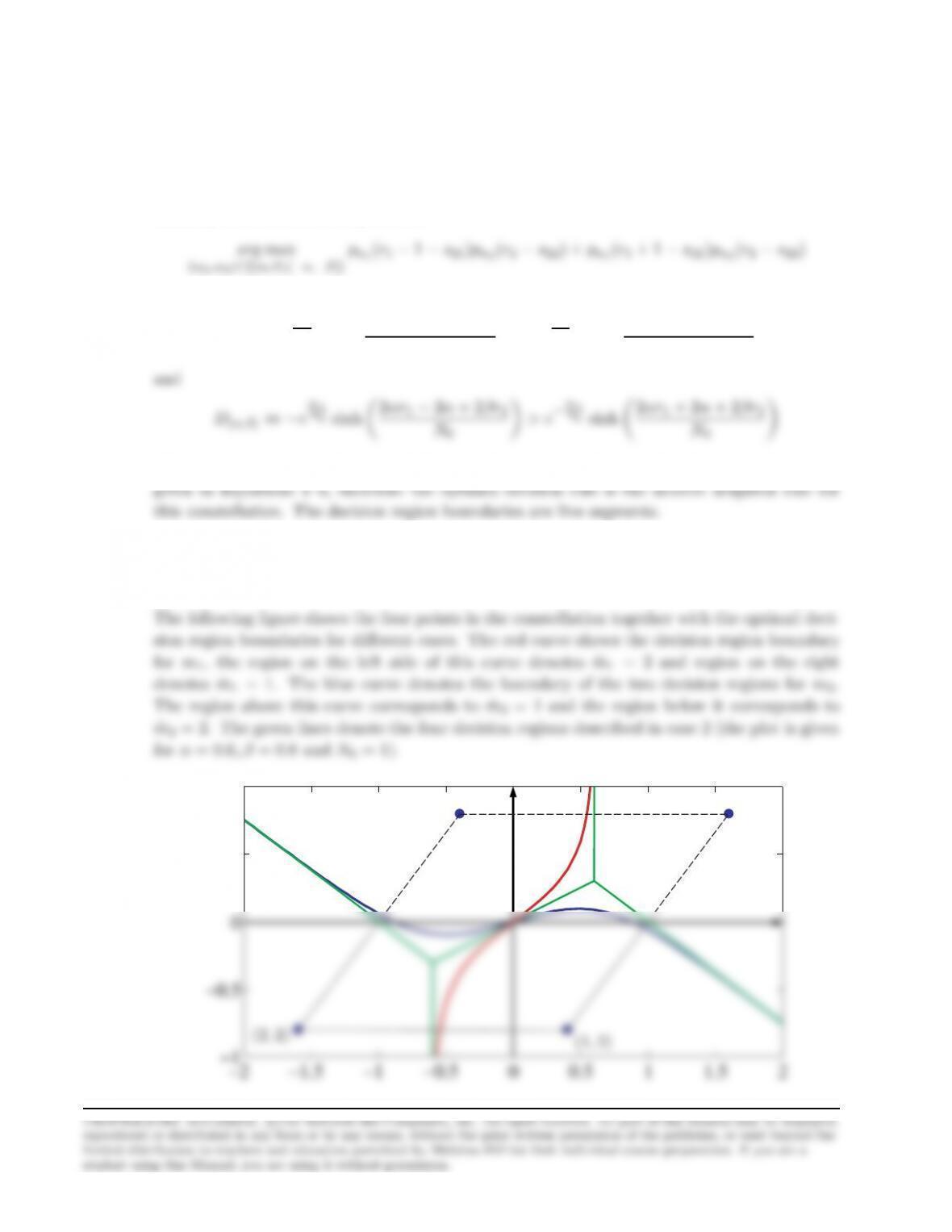
2. This case easy and straightforward. We have four equiprobable signals whose coordinates are

3. The “real” optimal detector is the one designed in part 1, since it minimizes each error

probability individually. However, it has a more complex structure due to nonlinear relations

that define the decision boundaries.

4. This is an example of a communication situation that even in the binary case one cannot

derive a closed form expression for the error probability. In case 2 we cannot find a closed

Problem 4.52

M

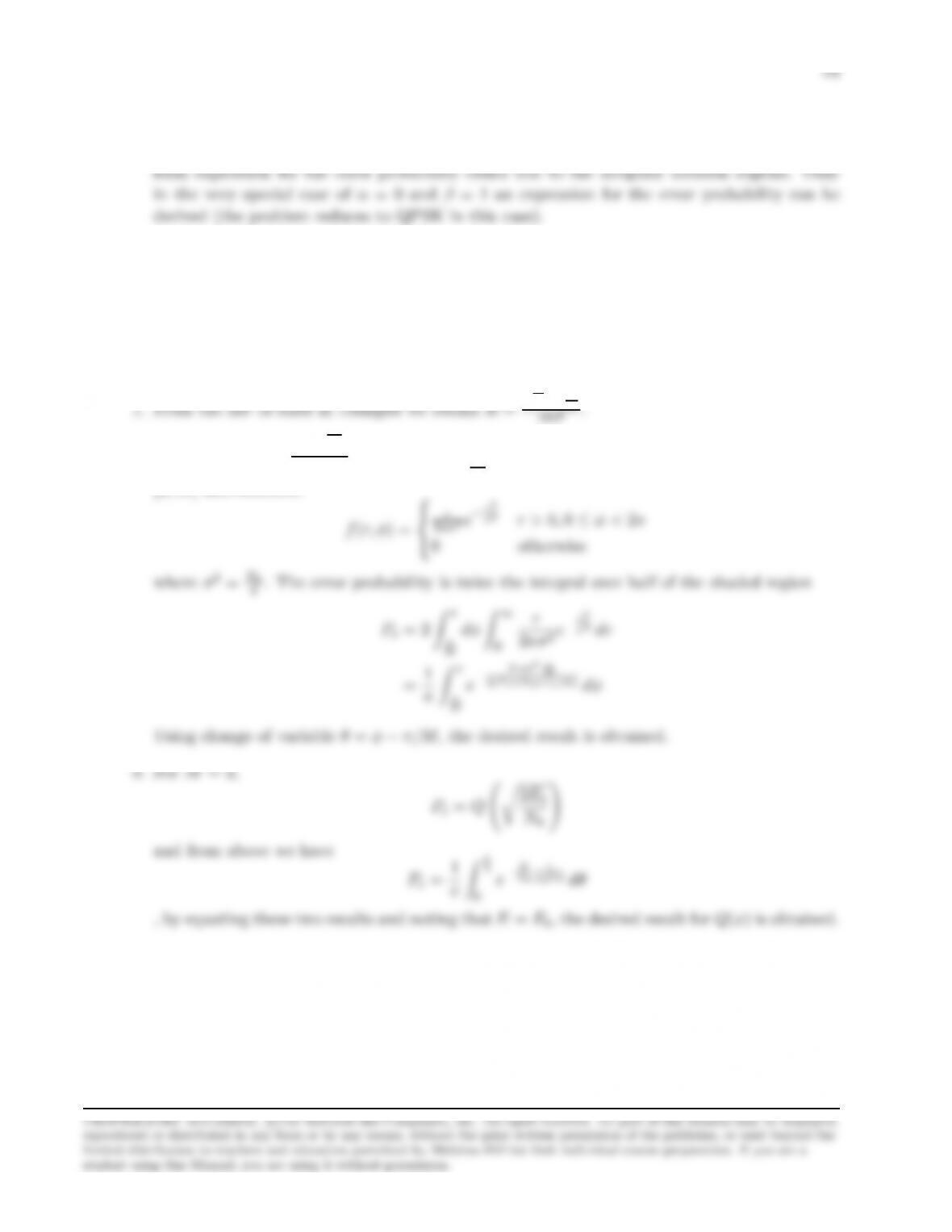
2. Let the origin be at √Ethen the error probability is P[(n1, n2)∈shaded area]. In polar

coordinates r=pn2

1+n2

2and φ= arctan n2

n1are independent with Rayleigh and uniform on

[0,2π] distributions.



r

σ2r > 0,0≤φ < 2π

Problem 4.53

55

1. We have to look for arg maxmp(r1,r2|sm) = arg maxmpn1(r1−sm)pn2(r2−sm) by the

independence of the noise processes. This reduces to arg maxmexp −|r1−sm|2

N01 −|r2−sm|2

N02 or

4. Here we are dealing with a one dimensional case and comparing

r1

N01

+r2

N02 pEm−Em

21

N01

+1

N02 >0

5. Of course α= 1 and rth =√Em. The detection rule is r1+r2>√Em. An error occurs

when n1+n2>√Em. But n1+n2is Gaussian with variance N0, hence Pe=QqEm

Problem 4.54

1. Since the two intervals are non-overlapping we can use two basis for representation of the

signal in the two intervals, the vector representation of the received signal will be (r1, r2) =

0

or

Z∞

0

e−(r1−1)2+(r2−a)2

N0e−ada > Z∞

0

e−(r1+1)2+(r2+a)2

N0e−ada

2. Since the amplitude of the multipath link is always positive, it always helps the decision. In

fact the system with multipath as described above cannot perform worse than the system

Problem 4.55

2. In this case the two signals are multiplied by √2 cos(2πfct+θ) by the demodulator and then

passed through a LPF (the √2 factor is introduced to keep energy intact). The output of the

Pb=Q cos θr2Eb

N0!

Problem 4.56

1. A change of variable of the form yi=Rxi, 1 ≤i≤nshows taht

Vn(R) = ZZ…

Z

dx1dx2. . . dxn=RnZZ…

Z

dy1dy2. . . dyn=BnRn

2. Note that

p(y) = 1

(2π)n/2e−kyk2

2

3. By spherical symmetry of the PDF p(y) is a function of the length of the vector yand not the

5. This follows directly from part 4 and

0

6. We introduce the change of variable u=r2/2, from which r dr =du and hence rn−1dr =

2n

2−1un

2−1du, hence

Using the result of part 5, we have

Problem 4.57

58

It is clear that dmin(C) = 1 and by 4.7-25,

Eavg/2D≈2

nV (R)ZRkxk2dx

=2

…ZL/2

(x2

1+x2

2+. . . x2

n)dx1dx2. . . dxn

n

X

6

3. From 4.7-40, we have

γs(R) = n[V(R)]1+ 2

n

12 RRkxk2dx

n

Problem 4.58

v(t) = Pk[Iku(t−2kTb) + jJku(t−2kTb−Tb)] where u(t) = 





sin πt

2Tb,0≤t≤Tb

0,o.w.





.Note

2Tb

Hence, v(t) may be expressed as :

59

The transmitted signal is :

kIksin π(t−2kTb)

2Tb

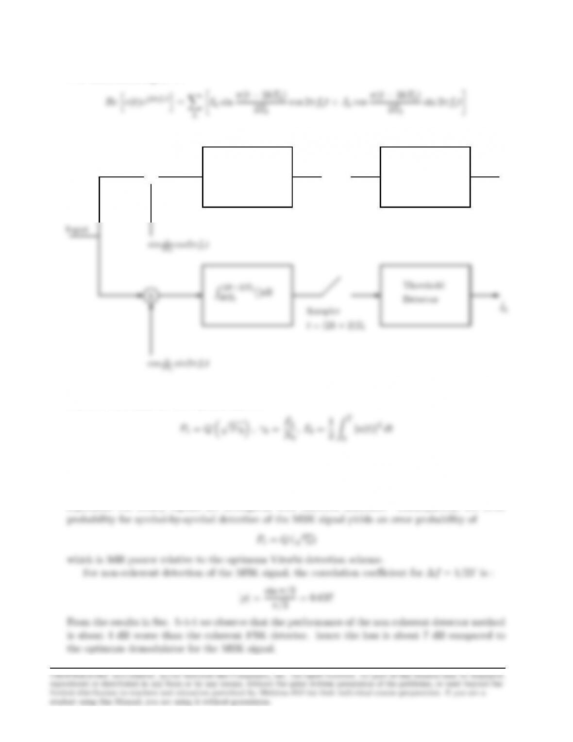
1.

✍✌

✎☞

✲ ✲ ✲ ✲

✻

Threshold

Detector

Sampler

t= (2k+ 2)Tb

XR(2k+2)Tb

2kTb()dt

ˆ

Ik

sin π

2Tbcos2πfct

Threshold

t= (2k+ 2)Tb

cos π

2Tbsin2πfct

Input

2. The offset QPSK signal is equivalent to two independent binary PSK systems. Hence for

coherent detection, the error probability is :

3. Viterbi decoding (MLSE) of the MSK signal yields identical performance to that of part (2).

4. MSK is basically binary FSK with frequency separation of ∆f= 1/2T. For this frequency

separation the binary signals are orthogonal with coherent detection. Consequently, the error

Problem 4.59

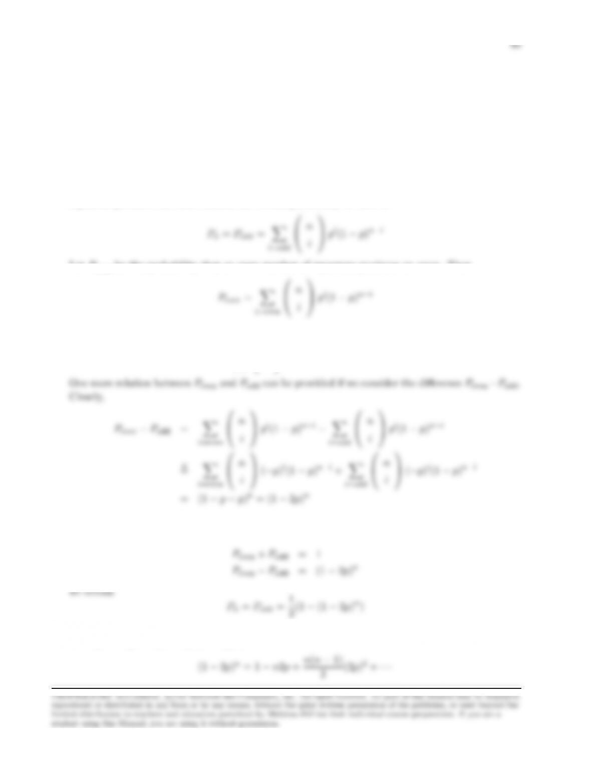
1. For nrepeaters in cascade, the probability of iout of nrepeaters to produce an error is given

by the binomial distribution

Pi=



n

i

pi(1 −p)n−i

However, there is a bit error at the output of the terminal receiver only when an odd number of

repeaters produces an error. Hence, the overall probability of error is

i=odd 

n

i

Let Peven be the probability that an even number of repeaters produces an error. Then

i=even 

n

i

and therefore,

Peven +Podd =

n

X

i=0 



n

i

pi(1 −p)n−i= (p+ 1 −p)n= 1

where the equality (a) follows from the fact that (−1)iis 1 for ieven and −1 when iis odd. Solving

the system

2. Expanding the quantity (1 −2p)n, we obtain

61

Since, p≪1 we can ignore all the powers of pwhich are greater than one. Hence,

Problem 4.60

The overall probability of error is approximated by (see 5-5-2)

P(e) = KQ “r2Eb

N0#

Problem 4.61

1. The antenna gain for a parabolic antenna of diameter Dis :

GR=ηπD

λ2

2. The effective radiated power is :

3. The received power is :

PR=PTGTGR

4πd

λ2= 2.995 ×10−9=−85.23 dB = −55.23 dBm

Problem 4.62

1. The antenna gain for a parabolic antenna of diameter Dis :

GR=ηπD

λ2

If we assume that the efficiency factor is 0.5, then with :

2. The effective radiated power is :

3. The received power is :

Problem 4.63

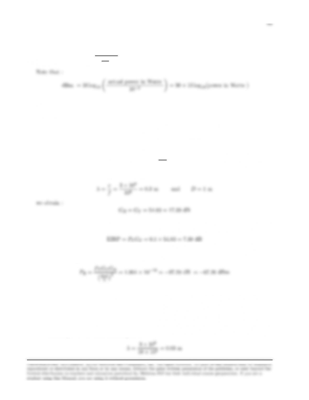
The wavelength of the transmitted signal is:

63

The gain of the parabolic antenna is:

λ2

0.032

The received power at the output of the receiver antenna is:

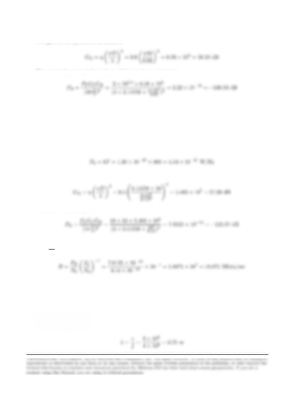
Problem 4.64

1. Since T= 3000K, it follows that

If we assume that the receiving antenna has an efficiency η= 0.5, then its gain is given by :

λ2

3×108

2×109!2

Hence, the received power level is :

2. If Eb

N0= 10 dB = 10, then

Problem 4.65

The wavelength of the transmission is :

64

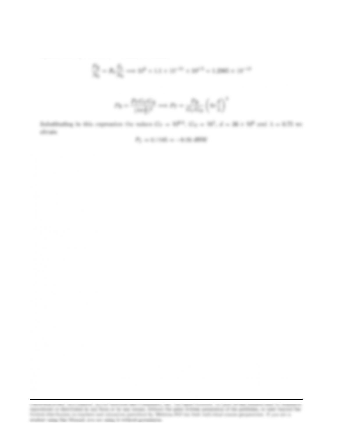
If 1 MHz is the passband bandwidth, then the rate of binary transmission is Rb=W= 106bps.

Hence, with N0= 4.1×10−21 W/Hz we obtain :

N0

The transmitted power is related to the received power through the relation (see 5-5-6) :