Problem 2.28
1) By Chernov bound, for t > 0,
P[X≥α]≤e−tαE[etX ] = e−tαΘX(t)
This is true for all t > 0, hence
2) Here
ln P[Sn≥α] = ln P[Y≥nα]≤ −max
t≥0[tnα −ln ΘY(t)]
where Y=X1+X2+···+Xn, and ΘY(t) = E[eX1+X2+···+Xn] = [ΘX(t)]n. Hence,
ΘX(t) = R∞
0etxe−xdx =1
1−tas long as t < 1. I(α) = maxt≥0(tα + ln(1 −t)), hence d
dt (tα + ln(1 −
Problem 2.29
For the central chi-square with ndegress of freedom :
ψ(jv) = 1
(1 −j2vσ2)n/2
Now : dψ(jv)
dv =jnσ2
(1 −j2vσ2)n/2+1 ⇒E(Y) = −jdψ(jv)
dv |v=0 =nσ2
22
where by definition : s2=Pn
i=1 m2
i.
dψ(jv)
dv =“jnσ2
(1 −j2vσ2)n/2+1 +js2
(1 −j2vσ2)n/2+2 #ejvs2/(1−j2vσ2)
Hence, E(Y) = −jdψ(jv)
dv |v=0 =nσ2+s2
Problem 2.30
The Cauchy r.v. has : p(x) = a/π
x2+a2,−∞ < x < ∞
a.
E(X) = Z∞
−∞
xp(x)dx = 0
since p(x) is an even function.
EX2=Z∞
−∞
x2p(x)dx =a
πZ∞
−∞
x2
x2+a2dx
b.
ψ(jv) = EjvX =Z∞
−∞
a/π
x2+a2ejvxdx =Z∞
−∞
a/π
(x+ja) (x−ja)ejvxdx
This integral can be evaluated by using the residue theorem in complex variable theory. Then, for

23
Therefore :
ψ(jv) = e−a|v|
Note: an alternative way to find the characteristic function is to use the Fourier transform rela-
tionship between p(x), ψ(jv) and the Fourier pair :
c
Problem 2.31
Since R0and R1are independent fR0,R1(r0, r1) = fR0(r0)fR1(r1) and
fR0,R1(r0, r1) =
r0r1
σ4I0µr1
σ2e−µ2
2σ2e−r2
1+r2
0
2σ2, r0, r1≥0
0,otherwise.
Now
P(R0> R1) = ZZ
r0>r1
f(r0, r1)dr1dr0
=Z∞
0
dr1Z∞
r1
f(r0, r1)dr0
=Z∞
fR1(r1)Z∞
fR0(r0)dr0dr1
r0
0
0
σ2I0µr1
σ2e−µ2+2r2
Now using the change of variable y=√2r1and letting s=µ
√2we obtain
P(R0> R1) = Z∞
y
√2σ2I0sy
2σ2dy
√2
y
24
y
Problem 2.32
1. The joint pdf of a, b is :
2πσ2e−1
2. u=√a2+b2, φ = tan −1b/a ⇒a=ucos φ, b =usin φThe Jacobian of the transformation is
∂a/∂u ∂a/∂φ
2πσ2e−1
where we have used the transformation :
M=qm2
r+m2
i
θ= tan −1mi/mr
⇒
mr=Mcos θ
mi=Msin θ
3.
pu(u) = Z2π
puφ(u, φ)dφ
Problem 2.33
a. Y=1
nPn
i=1 Xi, ψXi(jv) = e−a|v|
n
Y
n
Y
hold. The reason is that the Cauchy distribution does not have a finite variance.
Problem 2.34
Since Zand Zejθ have the same pdf, we have E[Z] = EZejθ=ejθE[Z] for all θ. Putting
Problem 2.35
Using Equation 2.6-29 we note that for the zero-mean proper case if W=ejθZ, it is suf-
Problem 2.36
Since Zis proper, we have E[(Z−E(Z))(Z−E(Z))t] = 0. Let W=AZ +b, then
Problem 2.37
We assume that x(t), y(t), z(t) are real-valued stochastic processes. The treatment of complex-
valued processes is similar.
a.
b. When x(t), y(t) are uncorrelated :
Rxy(τ) = E[x(t+τ)y(t)] = E[x(t+τ)] E[y(t)] = mxmy
c. When x(t), y(t) are uncorrelated and have zero means :
Problem 2.38
The power spectral density of the random process x(t) is :
Sxx(f) = Z∞
−∞
Rxx(τ)e−j2πfτ dτ =N0/2.
27
Problem 2.39
The power spectral density of X(t) corresponds to : Rxx(t) = 2BN0sin 2πBt
2πBt .From the result of
Problem 2.14 :
Ryy(τ) = R2
xx(0) + 2R2
xx(τ) = (2BN0)2+ 8B2N2
0sin 2πBt
2πBt 2
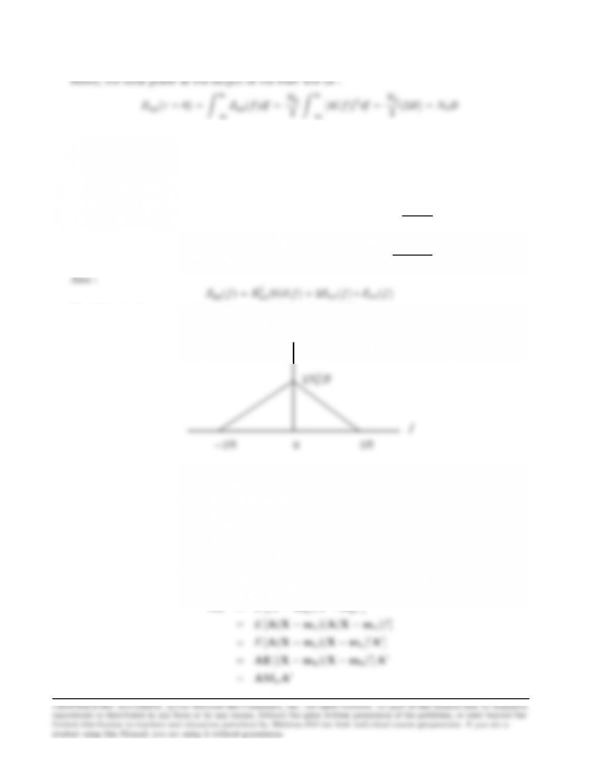
The following figure shows the power spectral density of Y(t) :
✻
✑✑✑✑✑✑✑
✑❩❩❩❩❩❩
❩
−2B0 2B
f
2N2
0B
(2BN0)2δ(f)
Problem 2.40
MX=E[(X−mx)(X−mx)′],X=
X1
X2
X3
,mxis the corresponding vector of mean values.
Then :
MY=E[(Y−my)(Y−my)′]
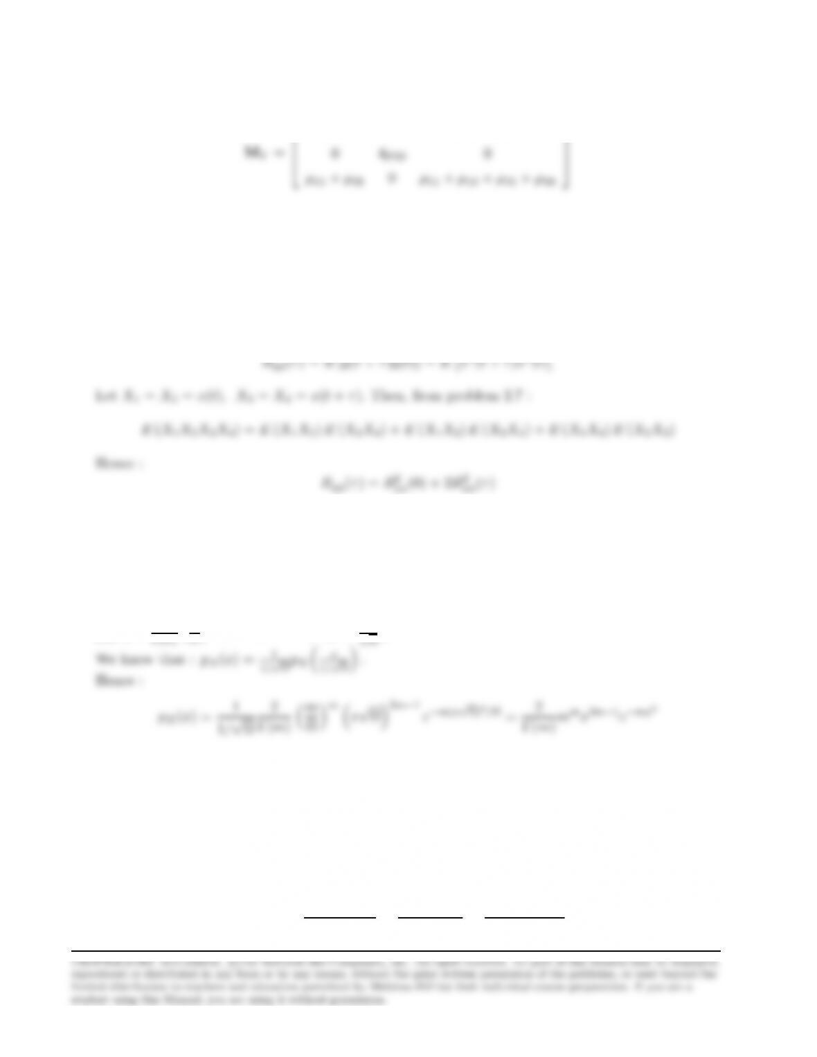
28
Hence :
µ11 0µ11 +µ13
Problem 2.41
Y(t) = X2(t), Rxx(τ) = E[x(t+τ)x(t)]
Problem 2.42
pR(r) = 2
Γ(m)m
Ωmr2m−1e−mr2/Ω, X =1
√ΩR
Problem 2.43
The transfer function of the filter is :
H(f) = 1/jωC
R+ 1/jωC =1
jωRC + 1 =1
j2πfRC + 1
29
a.
b.
Ryy(τ) = F−1{Sxx(f)}=σ2
RC Z∞
−∞
1
RC
(1
RC )2+ (2πf )2ej2πfτ df
Let : a=RC, v = 2πf. Then :
a/π
where the last integral is evaluated in the same way as in problem P-2.9 . Finally :
Problem 2.44
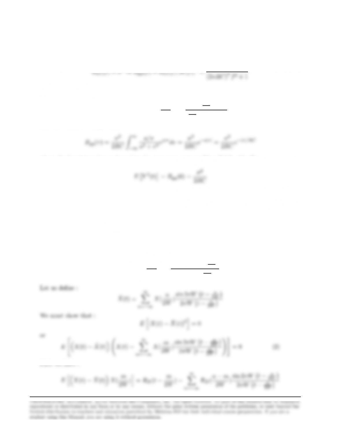
If SX(f) = 0 for |f|> W, then SX(f)e−j2πfa is also bandlimited. The corresponding autocorrelation
function can be represented as (remember that SX(f) is deterministic) :
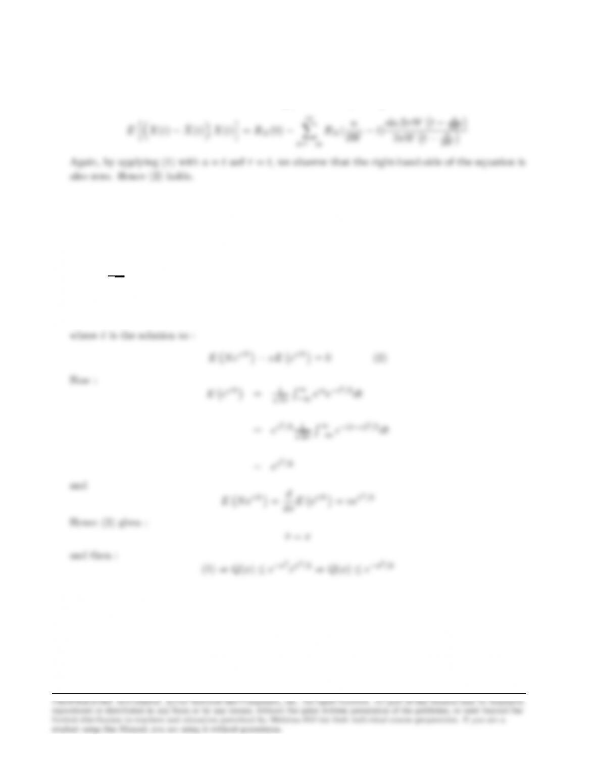
RX(τ−a) = ∞
X
n=−∞
RX(n
2W−a)sin 2πW τ−n
2W
2πW τ−n
2W(1)
First we have :
X
2W
30
But the right-hand-side of this equation is equal to zero by application of (1) with a=m/2W.
Since this is true for any m, it follows that EhX(t)−ˆ
X(t)ˆ
X(t)i= 0.Also
X
2W
Problem 2.45
Q(x) = 1
√2πR∞
xe−t2/2dt =P[N≥x],where Nis a Gaussian r.v with zero mean and unit variance.
From the Chernoff bound :
P[N≥x]≤e−ˆvxEeˆvN (1)
Problem 2.46
Since H(0) = P∞
−∞ h(n) = 0 ⇒my=mxH(0) = 0
31
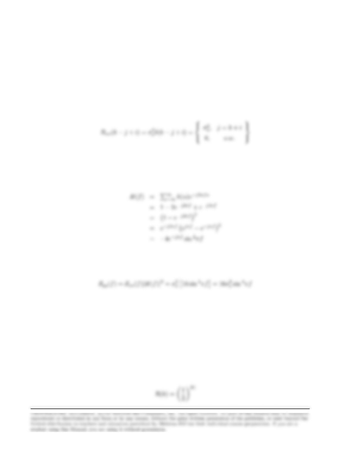
The autocorrelation of the output sequence is
Ryy(k) = X
iX
j
h(i)h(j)Rxx(k−j+i) = σ2
x
∞
X
i=−∞
h(i)h(k+i)
where the last equality stems from the autocorrelation function of X(n) :
σ2
x, j =k+i
0, o.w.
Hence, Ryy(0) = 6σ2
x, Ryy (1) = Ryy(−1) = −4σ2
x, Ryy (2) = Ryy (−2) = σ2
x, Ryy (k) = 0 otherwise.
Finally, the frequency response of the discrete-time system is :
which gives the power density spectrum of the output :
Problem 2.47