
Solutions Manual
for
Digital Communications, 5th Edition
(Chapter 16) 1
Prepared by
Kostas Stamatiou
March 12, 2008

2
Problem 16.1
gk(t) = ejθk
L−1
X
n=0
ak(n)p(t−nTc)
0
We also define as cross-correlation :
0
(a) For synchronous transmission, the received lowpass-equivalent signal r(t) is again given by
(16-3-9), while the log-likelihood ratio is :
Λ(b) = RT
0r(t)−PK
k=1 √Ekbkgk(t)
2dt
where rk=RT
0r(t)g∗
k(t)dt, and we assume that the information sequence {bk}is real. Hence, the
correlation metrics can be expressed in a similar form to (16-3-15) :
The only difference from the real-valued case of the text is that the correlation matrix Rsuses the
complex-valued cross-correlations given above :
ρ∗
ij(0), i ≤j
(b) Following the same procedure as in the text, we see that the correlator outputs are :
rk(i) = Z(i+1)T+τk
iT +τk
r(t)g∗
k(t−iT −τk)dt

RN=
Ra(0) Ra(−1) 0··· ···
Ra(1) Ra(0) Ra(−1) 0···
0..........
.
.
⇒
RN=
Ra(0) RaH(1) 0··· ···
Ra(1) Ra(0) RaH(1) 0···
0..........
.
.
where Ra(m) is a K×Kmatrix with elements :
Rkl(m) = Z∞
−∞
g∗
k(t−τk)gl(t+mT −τl)dt
Problem 16.2
The capacity per user CKis :
CK=1
KWlog 21 + P
W N0,lim
K→∞ CK= 0
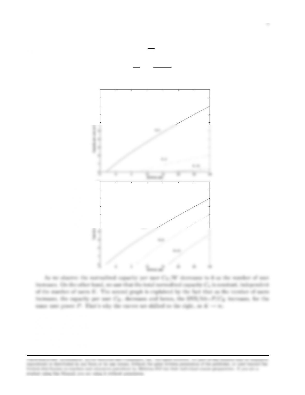
which is the relationship between the SNR and the normalized capacity per user. The relationship
between the normalized total capacity Cn=KCK
Wand the SNR is :
Eb
N0
=K2Cn−1
Cn
The corresponding plots for these last two relationships are given in the following figures :
−5 0 5 10 15 20 25 30
0
1
2
3
4
5
6
7
8
9
10
SNR/bit (dB)
Capacity per user per Hertz C_K/W
K=1
K=3
K=10
−5 0 5 10 15 20 25 30
0
1
2
3
4
5
6
7
8
9
10
SNR/bit (dB)
Total bit rate per Hertz C_n
K=1
K=3
K=10
As we observe the normalized capacity per user CK/W decreases to 0 as the number of user
increases. On the other hand, we saw that the total normalized capacity Cnis constant, independent
of the number of users K. The second graph is explained by the fact that as the number of users
increases, the capacity per user CK, decreases and hence, the SNR/bit=P/CKincreases, for the
same user power P. That’s why the curves are shifted to the right, as K→ ∞.
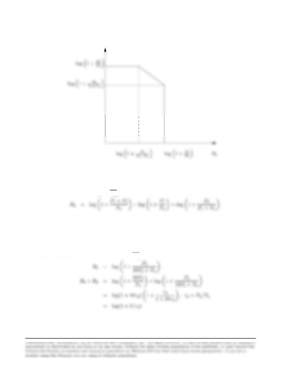
Problem 16.3

5
(a)
C1=aW log 21 + P1
aW N0
As avaries between 0 and 1, the graph of the points (C1, C2) is given in the following figure:
0 0.5 1 1.5 2 2.5
0
0.5
1
1.5
2
2.5
R_1
R_2
W=1, P1/N0=3, P2/N0=1
(b) Substituting P1/a =P2/(1 −a) = P1+P2,in the expression for C=C1+C2,we obtain :
C=C1+C2=Whalog 21 + P1+P2
Problem 16.4
(a) Since the transmitters are peak-power-limited, the constraint on the available power holds for
the allocated time frame when each user transmits. This is more restrictive that an average-power

6
Hence, in the peak-power limited system :
C1=aW log 21 + P1
W N0
(b) As avaries between 0 and 1, the graph of the points (C1, C2) is given in the following figure
0 0.5 1 1.5 2 2.5
0
0.5
1
1.5
2
2.5
R_1
R_2
W=1, P1/N0=3, P2/N0=1
Problem 16.5
(a) Since the system is average-power limited, the i-th user can transmit in his allocated time-frame
with peak-power Pi/ai,where aiis the fraction of the time that the user transmits.
Hence, in the average-power limited system :
C1=aW log 21 + P1/a
W N0
(b) As avaries between 0 and 1, the graph of the points (C1, C2) is given in the following figure

7
0 0.5 1 1.5 2 2.5
0
0.5
1
1.5
2
2.5
R_1
R_2
W=1, P1/N0=3, P2/N0=1
(c) We note that the expression for the total capacity is the same as that of the FDMA in Problem
16.2. Hence, if the time that each user transmits is proportional to the transmitter’s power :
P1/a =P2/(1 −a) = P1+P2,we have :
Problem 16.6
(a) We have
r1=ZT
0
r(t)g1(t)dt

8
(b) We have E[n1] (= m1) = E[n2] (= m2) = 0. Hence
In the same way, σ2
1=E[n2
1] = N0
2. The covariance is equal to
µ12 =E[n1n2]−E[n1]E[n2] = E[n1n2]
(c) Given b1and b2, then (r1,r2) follow the pdf of (n1,n2) which are jointly Gaussian with a
pdf given by (2-1-150) or (2-1-156). Using the results from (b)
p(r1, r2|b1, b2) = p(n1, n2)
1−2ρx1x2+x2
2
Problem 16.7
We use the result for r1, r2from Problem 5.6 (a) (or the equivalent expression (16.3-40)). Then,
assuming b1= 1 was transmitted, the probability of error for b1is
P1=P(error1|b2= 1)P(b2= 1) + P(error1|b2=−1)P(b2=−1)
=Qq2(√E1+ρ√E2)2
N01
2+Qq2(√E1−ρ√E2)2
N01
2

Problem 16.8
(a)
P(b1, b2|r(t),0≤t≤T) = p(r(t),0≤t≤T|b1, b2)P(b1, b2)
p(r(t),0≤t≤T)
But P(b1, b2) = P(b1)P(b2) = 1/4 for any pair of (b1, b2) and p(r(t),0≤t≤T) is independent
of (b1, b2). Hence
(b) Sufficient statistics for r(t),0≤t≤Tare the correlator outputs r1, r2at t=T. From
Problem 16.6 the joint pdf of r1, r2given b1, b2is
p(r1, r2|b1, b2) = 1
2πN0
2p1−ρ2exp −x2
1−2ρx1x2+x2
2
2(1 −ρ2)
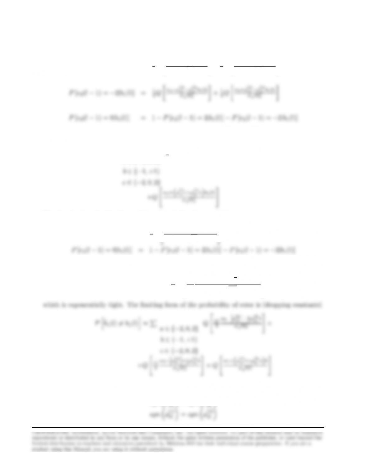
Problem 16.9
(a)
P(b1|r(t),0≤t≤T) = P(b1|r1, r2)
=P(b1, b2= 1|r1, r2) + P(b1, b2=−1|r1, r2)

10
From Problem 15.6 the joint pdf of r1, r2given b1, b2is
p(r1, r2|b1, b2) = 1
2πN0
2p1−ρ2exp −x2
1−2ρx1x2+x2
2
2(1 −ρ2)
arg maxb1P(b1|r(t),0≤t≤T) = arg max hexp √E1b1r1+√E2r2−√E1E2b1ρ
N0
+ exp √E1b1r1−√E2r2+√E1E2b1ρ
(b) From part(a)
b1= 1 ⇔√E1r1
2√E1
cosh(√E2r2−√E1E2ρ
N0)
Problem 16.10
As N0→0, the probability in expression (16.3-62) will be dominated by the term which has the
smallest argument in the Q function. Hence
effective SN R = min
bjh√Ek+Pj6=kpEjbjρjki2
N0

Problem 16.11
The probability that the ML detector makes an error for the first user is :
P1=Pb1,b2P(ˆ
b16=b1|b1, b2)(P(b1, b2)
=1
4(P[++ → −+] + P[++ → −−])
where P[b1b2→ˆ
b1ˆ
b2] denotes the probability that the detector chooses (ˆ
b1ˆ
b2) conditioned
on (b1, b2) having being transmitted. Due to the symmetry of the decision statistic, the above
relationship simplifies to
From Problem 16.8 we know that the decision of this detector is based on
(ˆ
b1,ˆ
b2) = arg max S(b1, b2) = pE1b1r1+pE2b2r2−pE1E2b1b2ρ
Hence, P[−− → +−] can be upper bounded as
P[−− → +−]≤P[S(−−)< S(+−)|(−−) transmitted]
This is a bound and not an equality since the if S(−−)< S(+−) then (−−) is not chosen, but
not necessarily in favor of (+−); it may have been in favor of (++) or (−+).
The last bound is easy to calculate :
P[S(−−)< S(+−)|(−−)transmitted]
Similarly, for the other three terms of (1) we obtain :
P[−− → ++] ≤P[S(−−)< S(++)|(−−) transmitted]

12
By adding the four terms we obtain
P1≤Qq2E1
N0+1
2Qq2E1+E2−2√E1E2ρ
N0
But we note that if ρ≥0, the last term is negligible, while if ρ≤0, then the second term is
negiligible. Hence, the bound can be written as
N0!+1
2Q
N0
Problem 16.12
(a) We have seen in Prob. 16.11 that the probability of error for user 1 can be upper bounded by
N0!+1
2Q
N0
As N0→0 the probability of error will be dominated by the Qfunction with the smallest
argument. Hence
(b) The plot of the asymptotic efficiencies is given in the following figure


Problem 16.14
(a) The matrix Rsis
Rs=
1ρ
ρ1
Hence the linear transformation A0for the two users will be
2I−1
1 + N0
2ρ
ρ1 + N0
2
−1
1 + N0
22−ρ2
1 + N0
2−ρ
−ρ1 + N0
2
(b) The limiting form of A0, as N0→0 is obviously
A0→1
1−ρ2
1−ρ
−ρ1
(c) The limiting form of A0, as N0→ ∞ is
N0
N0
1 0
Problem 16.15
(a) The performance of the receivers, when no post-processing is used, is the performance of the
(b) Since : y1(l) = b1(l)w1+b2(l)ρ(1)
12 +b2(l−1)ρ(1)
21 +n, the decision variable z1(l),for the first
user after post-processing, is equal to :
15
orthogonal when conditioned on b1(l).The distribution of e2(l−1),conditioned on b1(l) is :
P[e2(l−1) = +2|b1(l)] = 1
4Qw2+ρ(2)
12 +ρ(2)
21 b1(l)
σ√w2+1
4Qw2−ρ(2)
12 +ρ(2)
21 b1(l)
σ√w2
12 −ρ(2)
21 b1(l)
12 −ρ(2)
21 b1(l)
The distribution of e2(l),given b1(l),is similar, just exchange ρ(2)
12 with ρ(2)
21 .Then, the probability
of error for user 1 is :
Phˆ
b1(l)6=b1(l)i=Pa∈ {−2,0,2}
1
2P[e2(l−1) = a|b1(l) = b]P[e2(l) = c|b1(l) = b]×
12 c+ρ(1)
21 a”b1(l)
The distribution of e2(l−1),conditioned on b1(l),when σ→0 is :
P[e2(l−1) = a|b1(l)] ≈1
4Q“w2−˛
˛
˛ρ(2)
12 ˛
˛
˛+aρ(2)
21 b1(l)/2
σ√w2#, a =±2
This distribution may be concisely written as :
P[e2(l−1) = a|b1(l)] ≈1
4Q
|a|
2
w2−ρ(2)
12 +a
2ρ(2)
21 b1(l)
σ√w2
(c) Consider the special case :
sgn ρ(1)

16
as would occur for far-field transmission (this case is the most prevalent in practice ; other cases
follow similarly). Then, the slowest decaying term corresponds to either :
sgn bρ(1)
21 a=sgn bρ(1)
12 c=−1
for which the resulting term is :
12 +ρ(2)
21
12 +ρ(1)
21
σ2
rw2
w1−ρ(2)
√w1√w2
σ2
w1
or the case when a=c= 0 for which the term is :
Qrw1
σ2
Therefore, the asymptotic efficiency of this detector is :
1,max2(0,qw2
w1−˛
˛
˛ρ(2)
12 ˛
˛
˛+˛
˛
˛ρ(2)
21 ˛
˛
˛
√w1√w2)+ max2(0,1−2max“˛
˛
˛ρ(1)
12 ˛
˛
˛,˛
˛
˛ρ(1)
21 ˛
˛
˛”
w1),
2 max2(0,qw2
w1−˛
√w1√w2)+ max2(0,1−2max“˛
w1)
Problem 16.16
(a) The normalized offered traffic per user is : Guser =λ·Tp=1
Problem 16.17
A, the average normalized rate for retransmissions, is the total rate of transmissions (G) times the

Problem 16.18
(a) Since the number of arrivals in the interval T, follows a Poisson distribution with parameter
Problem 16.19
(a) Since the average number of arrivals in 1 sec is E[k] = λT = 10,the average time between
Problem 16.20

Problem 16.21
(d) For non-persistent CDMA :
S=Ge−aG
G(1 + 2a) + e−aG
Problem 16.22
The capacity region for K= 2 users is shown below:
19
R2
(a)
R1= log 1 + P1
No
(b) P1= 10P2. Then,
R1= log 1 + P1
No

20
(c)
R1= log 1 + P1
P2+No