
Solutions Manual
for
Digital Communications, 5th Edition
(Chapter 10) 1
Prepared by
Kostas Stamatiou
January 15, 2008
2
Problem 10.1
(a)
F(z) = 4
5+3
5z−1⇒X(z) = F(z)F∗(z−1) = 1 + 12
25 z+z−1
Hence :
Γ=
112
25 0
12
25 112
25
012
25 1
ξ=
3/5
4/5
0
−0.456
(b) The eigenvalues of the matrix Γare given by :
|Γ−λI|= 0 ⇒
1−λ0.48 0
0.48 1 −λ0.48
= 0 ⇒λ= 1,0.3232,1.6768
The step size ∆ should range between :
(c) Following equations (10-3-3)-(10-3-4) we have :
ψ=
1 0.48
0.48 0.64
, ψ
c−1
c0
=
0.6
0.8
⇒
Problem 10.2
(a)
(b) From (10-1-31) :
J∆= ∆2Jmin
3
X
k=1
λ2
k
1−(1 −∆λk)2≈1
2∆Jmin
3
X
k=1
λk
1 + N0
(c) Let C′=VtC, ξ′=Vtξ, where Vis the matrix whose columns form the eigenvectors of the
covariance matrix Γ(note that Vt=V−1).Then :
C(n+1) = (I−∆Γ)C(n)+ ∆ξ⇒
C(n+1) =I−∆VΛV−1C(n)+ ∆ξ⇒
which is a set of three de-coupled difference equations (de-coupled because Λ is a diagonal matrix).
Hence, we can write :
k=ξ′
λk
or going back to matrix form :
C′=Λ−1ξ′⇒
which agrees with the result in Probl. 9.49(a).
Problem 10.3
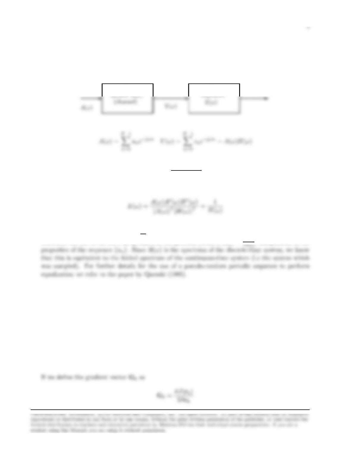
Suppose that we have a discrete-time system with frequency response H(ω); this may be equalized
by use of the DFT as shown below :
an
System H(ω)
yn
Equalizer
output
N−1
X
n=0
N−1
X
n=0
Let :
E(ω) = A(ω)Y∗(ω)
|Y(ω)|2
Then by direct substitution of Y(ω) we obtain :
If the sequence {an}is sufficiently padded with zeros, the N-point DFT simply represents the
values of E(gw) and H(ω) at ω=2π
Nk=ωk,for k= 0,1, …N −1 without frequency aliasing.
Therefore the use of the DFT as specified in this problem yields E(ωk) = 1
Problem 10.4
The MSE performance index at the time instant kis
J(ck) = E
N
X
n=−N
ck,nvk−n−Ik
2
5
then its l−th element is
Gk,l =ϑJ(ck)
2ϑck,l
=1
2E“2 N
X
ck,nvk−n−Ik!v∗
k−l#
Problem 10.5
The tap-leakage LMS algorithm is :
C(n+ 1) = wC(n) + ∆ǫ(n)V∗(n) = wC(n) + ∆ (ΓC(n)−ξ) = (wI−∆Γ)C(n)−∆ξ
and since ∆ >0,the convergence criterion is :
Problem 10.6
The estimate of g can be written as : ˆg=h0x0+… +hM−1xM−1=xTh,where x,hare column
vectors containing the respective coefficients. Then using the orthogonality principle we obtain the
optimum linear estimator h:

6
or :
hopt =R−1
xx c
where we have used the fact that gand ware independent, and that E[g] = 0.Also, the column
Problem 10.7
(a) The time-update equation for the parameters {Hk}is :
H(n+1)
k=H(n)
k+ ∆ǫ(n)y(n)
k
where nis the time-index, kis the filter index, and y(n)
kis the output of the k-th filter with transfer
function : 1−z−M/1−ej2πk/M z−1as shown in the figure below :
– –
?66
y0(n)
H0
z−1
+X
+
–
– –
y1(n)
+X
+
– –
?66
yM−1(n)
HM−1
z−1
+X
+
–
ej2π(M−1)/M
CCCCCCCCCCCC
1/M z−M
.
.
Parallel Bank of Single −Pole Filters

7
(b) It is straightforward to prove that the transfer function of the k-th filter in the parallel bank
has a resonant frequency at fk= 2πk
Problem 10.8
(a) The gradient of the performance index Jwith respect to his : dJ
dh = 2h+ 40.Hence, the time
update equation becomes :
hn+1 =hn−1
2∆(2hn+ 40) = hn(1 −∆) −20∆
(b) We note that Jhas a minimum at h=−20,with corresponding value : Jmin =−372.To
illustrate the convergence of the algorithm let’s choose : ∆ = 1/2.Then : hn+1 =hn/2−10,and,
using induction, we can prove that :
X
k=0 1
where h0is the initial value for h. Then, as n→ ∞,the dependence on the initial condition h0
vanishes and hn→ −10 1
1−1/2=−20,which is the desired value. The following plot shows the
expression for Jas a function of n, for ∆ = 1/2 and for various initial values h0.
h0=−25
h0=−30
h0=0
0 2 4 6 8 10 12 14 16 18 20
−400
−350
−250
−200
−150
−100
−50
0
50
Iteration n
J(n)
PROPRIETARY MATERIAL. c
The McGraw-Hill Companies, Inc. All rights reserved. No part of this Manual may be displayed,
reproduced or distributed in any form or by any means, without the prior written permission of the publisher, or used beyond the
limited distribution to teachers and educators permitted by McGraw-Hill for their individual course preparation. If you are a
student using this Manual, you are using it without permission.
Problem 10.9
The linear estimator for xcan be written as : ˆx(n) = a1x(n−1)+a2x(n−1) = [x(n−1) x(n−2)]
a1
a2
.
Using the orthogonality principle we obtain :
E
x(n−1)
x(n−2)
ǫ
= 0 ⇒E
x(n−1)
x(n−2)
x(n)−[x(n−1) x(n−2)]
a1
a2
= 0
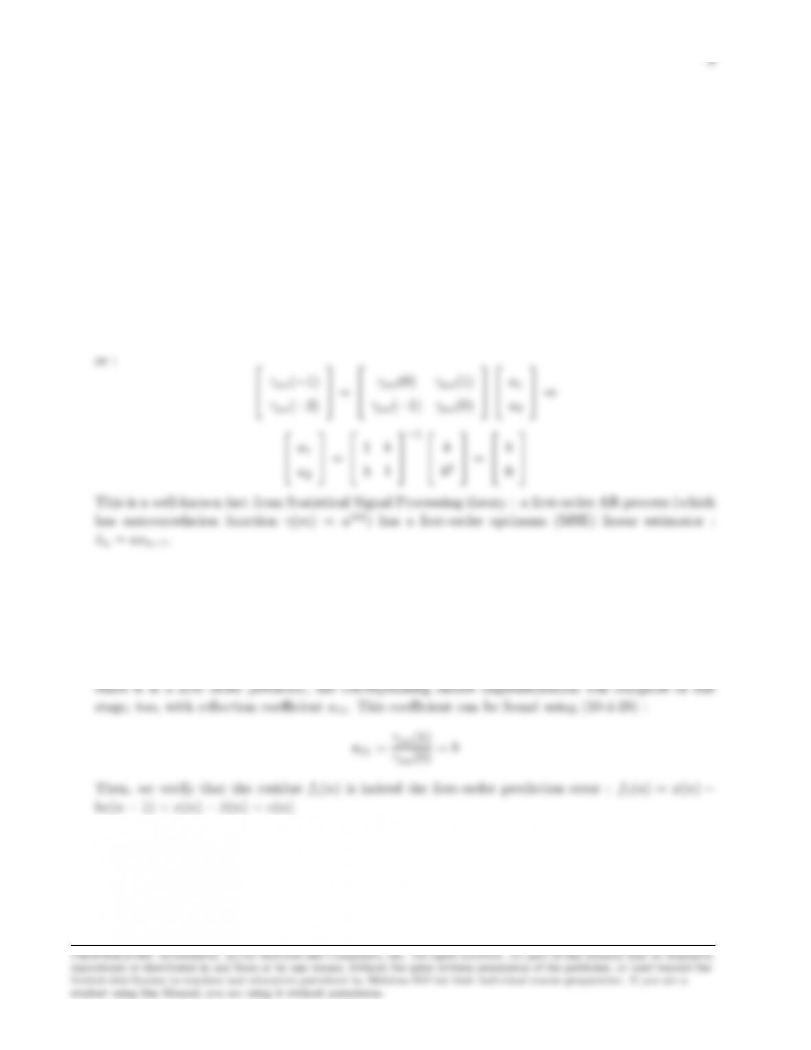
Problem 10.10
In Probl. 10.9 we found that the optimum (MSE) linear predictor for x(n),is ˆx(n) = bx(n−1).
Problem 10.11
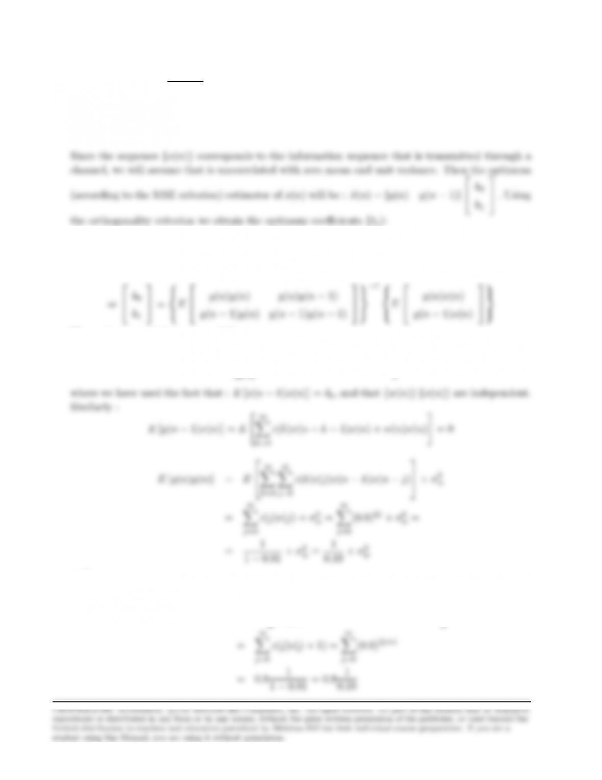
9
The system C(z) = 1
1−0.9z−1has an impulse response : c(n) = (0.9)n, n ≥0.Then, we write the
input y(n) to the adaptive FIR filter :
y(n) = ∞
X
k=0
c(k)x(n−k) + w(n)
E
y(n)
y(n−1)
ǫ
= 0 ⇒E
y(n)
y(n−1)
x(n)−[y(n)y(n−1)]
b0
b1
= 0
b0
b1
y(n)y(n)y(n)y(n−1)
y(n−1)y(n)y(n−1)y(n−1)
−1
y(n)x(n)
y(n−1)x(n)
The various correlations are as follows :
E[y(n)x(n)] = E“∞
X
c(k)x(n−k)x(n) + w(n)x(n)#=c(0) = 1
1−0.81 +σ2
0.19 +σ2
and :
E[y(n)y(n−1)] = E
∞
X
k=0
∞
X
j=0
c(k)c(j)x(n−k)x(n−1−j)
X
X
10
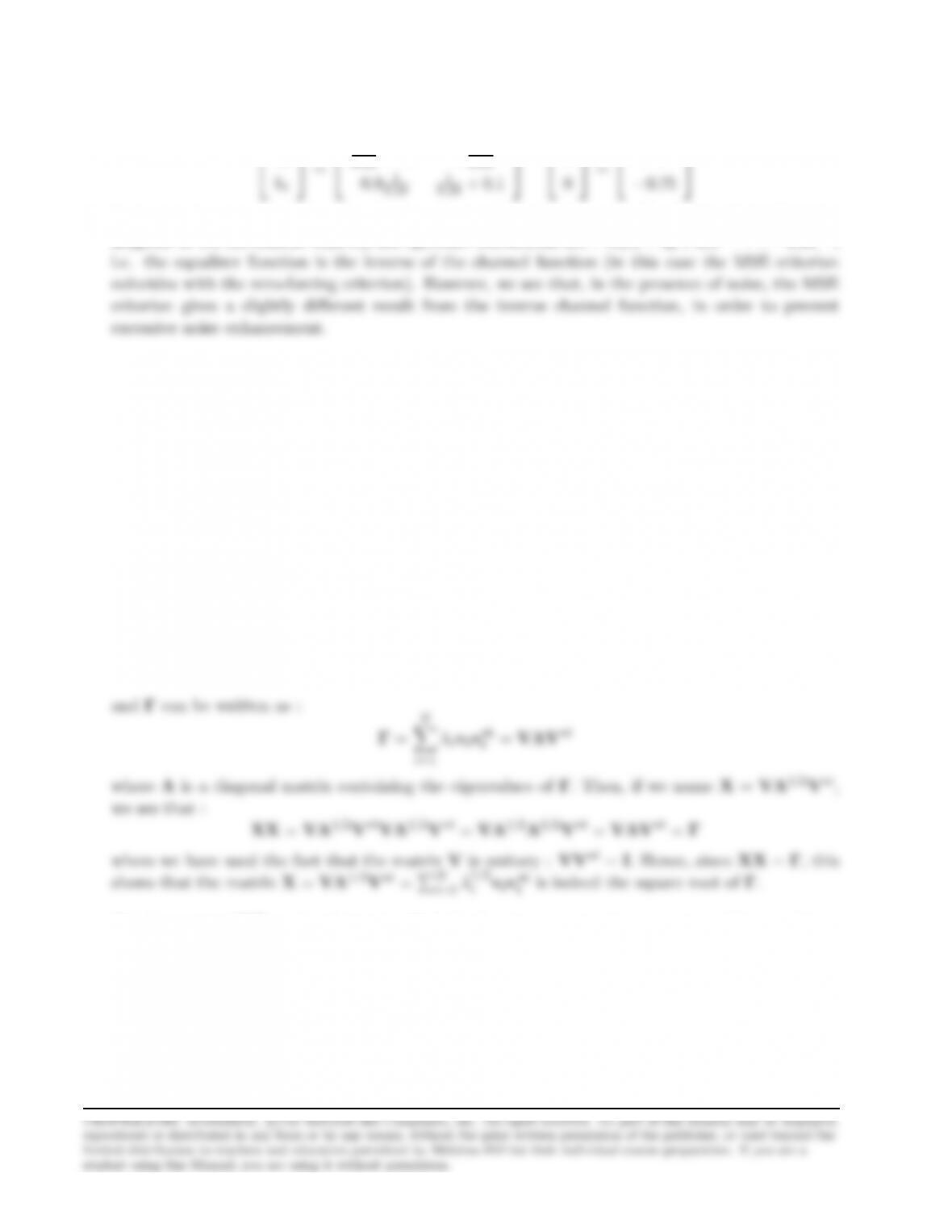
Hence :
b0
b1
1
0.91
0.19
1
0.19 + 0.1
−1
1
0
0.85
−0.75
It is interesting to note that in the absence of noise (i.e when the term σ2
w= 0.1 is missing from the
diagonal of the correlation matrix), the optimum coefficients are : B(z) = b0+b1z−1= 1 −0.9z−1,
Problem 10.12
(a) If we denote by Vthe matrix whose columns are the eigenvectors {vi}:
V= [v1|v2|…|vN]
then its conjugate transpose matrix is :
V∗t=
v∗t
1
v∗t
2
…
v∗t
N
(b) To compute Γ1/2,we first determine V,Λ(i.e the eigenvalues and eigenvectors of the correlation
matrix). Then :
Γ1/2=
N
X
i=1
λ1/2
iviv∗t
i=VΛ1/2V∗t