CHAPTER 11
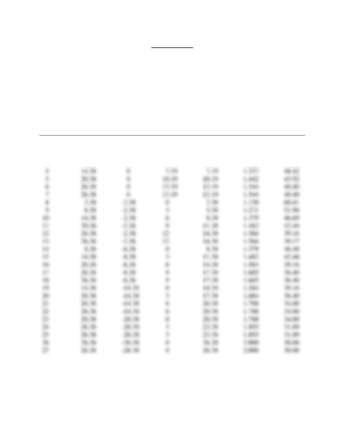
11.1 The solution is given in the following table and graph of the contour. The point numbers
in the table correspond to the numbered points on the graph.
Point K– = K+ = = = M =
# + – ½(K–+K+) ½(K–+K+) (deg)
(deg) (deg) (deg) (deg)
1 0.38 0 0.19 0.19 1.026 77.14
2 2.38 0 1.19 1.19 1.092 66.29
3 8.38 0 4.19 4.19 1.225 54.88

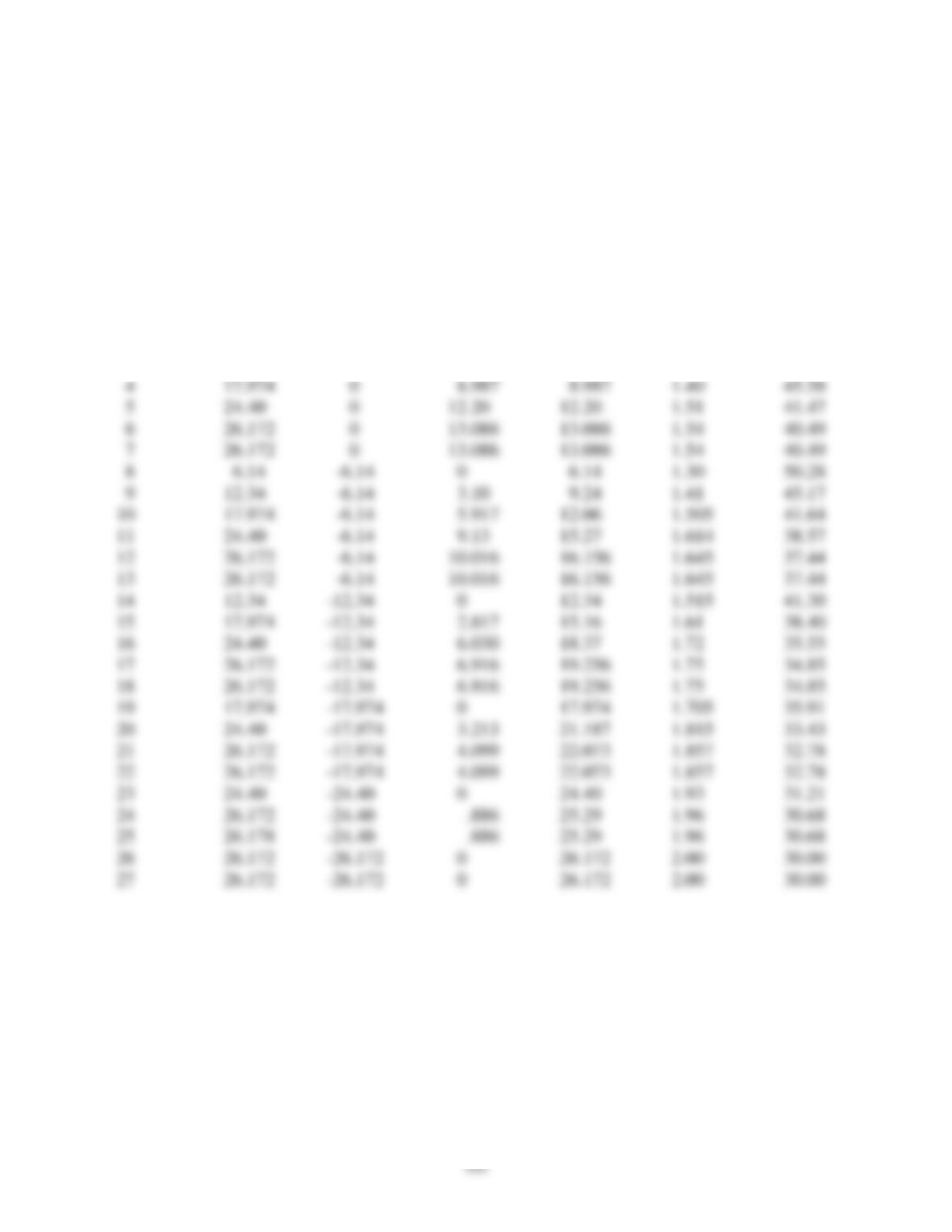
11.2 The solution is given in the same format as Problem 11.1.
Point K– = K+ = = = M =
# + – ½(K–+K+) ½(K–+K+) (deg)
(deg) (deg) (deg) (deg)
1 .975 0 0.4874 0.4874 1.05 72.25
2 6.14 0 3.07 3.07 1.18 57.94
3 12.34 0 6.17 6.17 1.30 50.28

105
11.3 Because of the curved shock wave attached to the tip of the body, the flowfield between
the body and the shock is rotational. However, to illustrate the application of the method of
The solution is carried out in the following steps:
106
5. At this stage, all properties have been found along the left-running characteristic 6-10.
Repeat the above process for the next downstream left-running characteristic, 11-14. You will