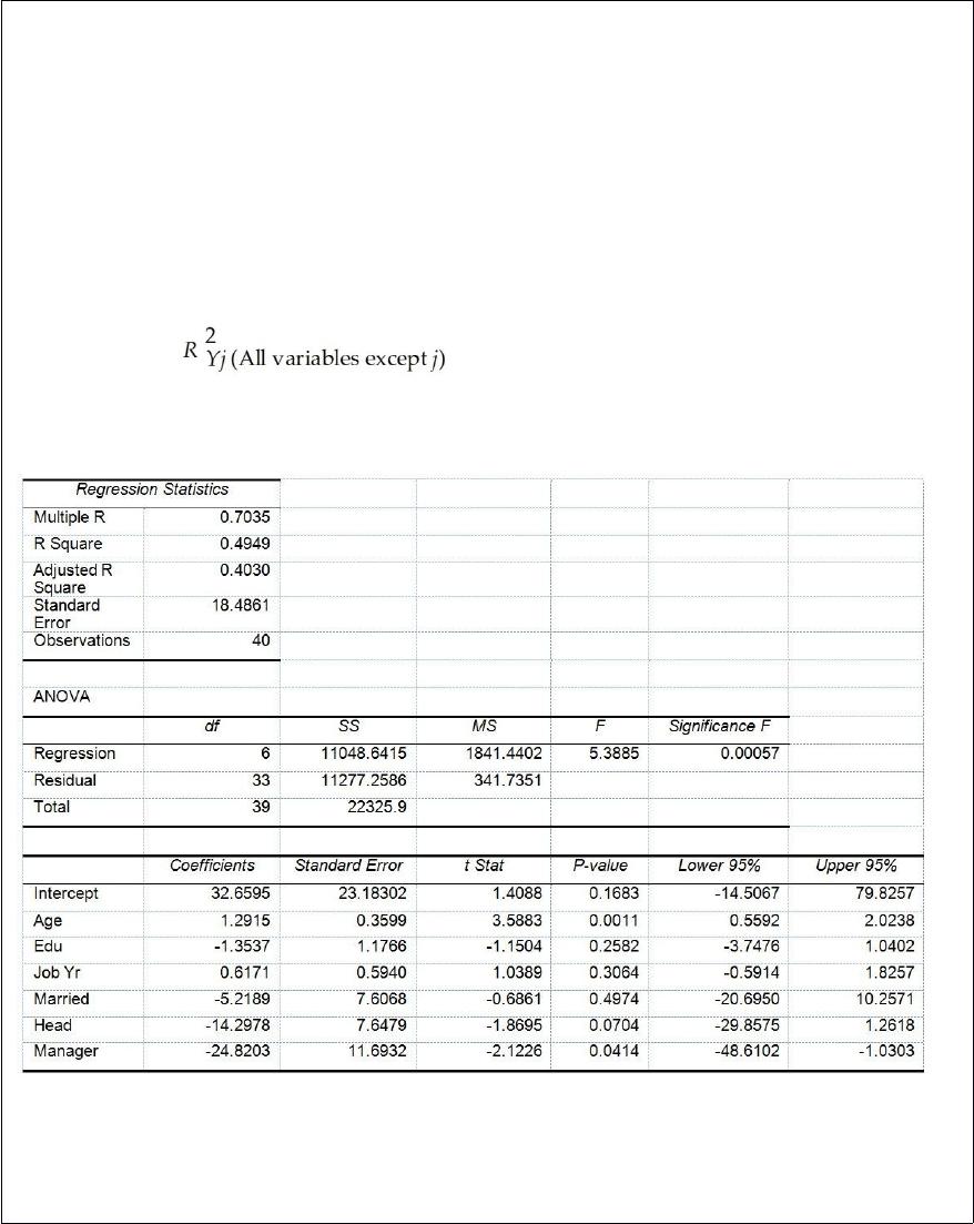
TABLE 17-10
Given below are results from the regression analysis where the dependent variable is
the number of weeks a worker is unemployed due to a layoff (Unemploy) and the
independent variables are the age of the worker (Age), the number of years of education
received (Edu), the number of years at the previous job (Job Yr), a dummy variable for
marital status (Married: 1 = married, 0 = otherwise), a dummy variable for head of
household (Head: 1 = yes, 0 = no) and a dummy variable for management position
(Manager: 1 = yes, 0 = no). We shall call this Model 1. The coefficient of partial
determination ( ) of each of the 6 predictors are, respectively,
0.2807, 0.0386, 0.0317, 0.0141, 0.0958, and 0.1201.
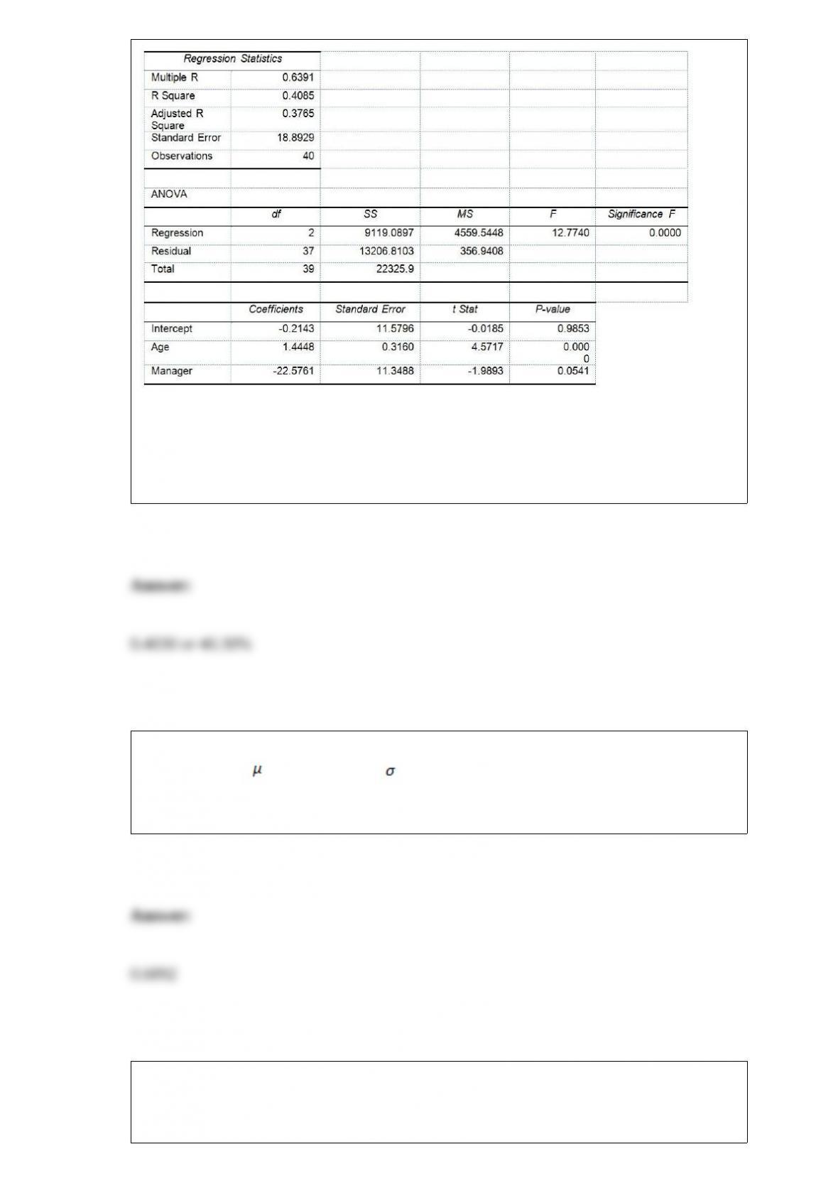
Model 2 is the regression analysis where the dependent variable is Unemploy and the
independent variables are Age and Manager. The results of the regression analysis are
given below:
Referring to Table 17-10, Model 1, ________ of the variation in the number of weeks a
worker is unemployed due to a layoff can be explained by the six independent variables
after taking into consideration the number of independent variables and the number of
observations.
The amount of tea leaves in a can from a particular production line is normally
distributed with = 110 grams and = 25 grams. What is the probability that a
randomly selected can will contain less than 100 grams or more than 120 grams of tea
leaves?
Suppose Z has a standard normal distribution with a mean of 0 and standard deviation
of 1. So, 96% of the possible Z values are between ________ and ________
(symmetrically distributed about the mean).
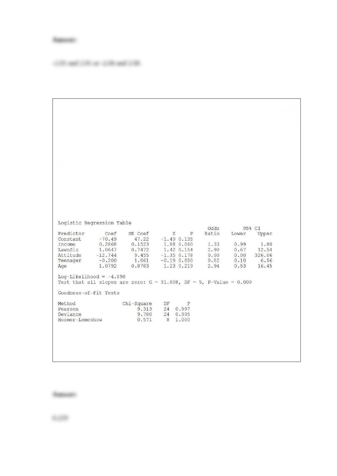
TABLE 17-12
The marketing manager for a nationally franchised lawn service company would like to
study the characteristics that differentiate home owners who do and do not have a lawn
service. A random sample of 30 home owners located in a suburban area near a large
city was selected; 15 did not have a lawn service (code 0) and 15 had a lawn service
(code 1). Additional information available concerning these 30 home owners includes
family income (Income, in thousands of dollars), lawn size (Lawn Size, in thousands of
square feet), attitude toward outdoor recreational activities (Attitude 0 = unfavorable, 1
= favorable), number of teenagers in the household (Teenager), and age of the head of
the household (Age).
The Minitab output is given below:
Referring to Table 17-12, what is the p-value of the test statistic when testing whether
Age makes a significant contribution to the model in the presence of the other
independent variables?
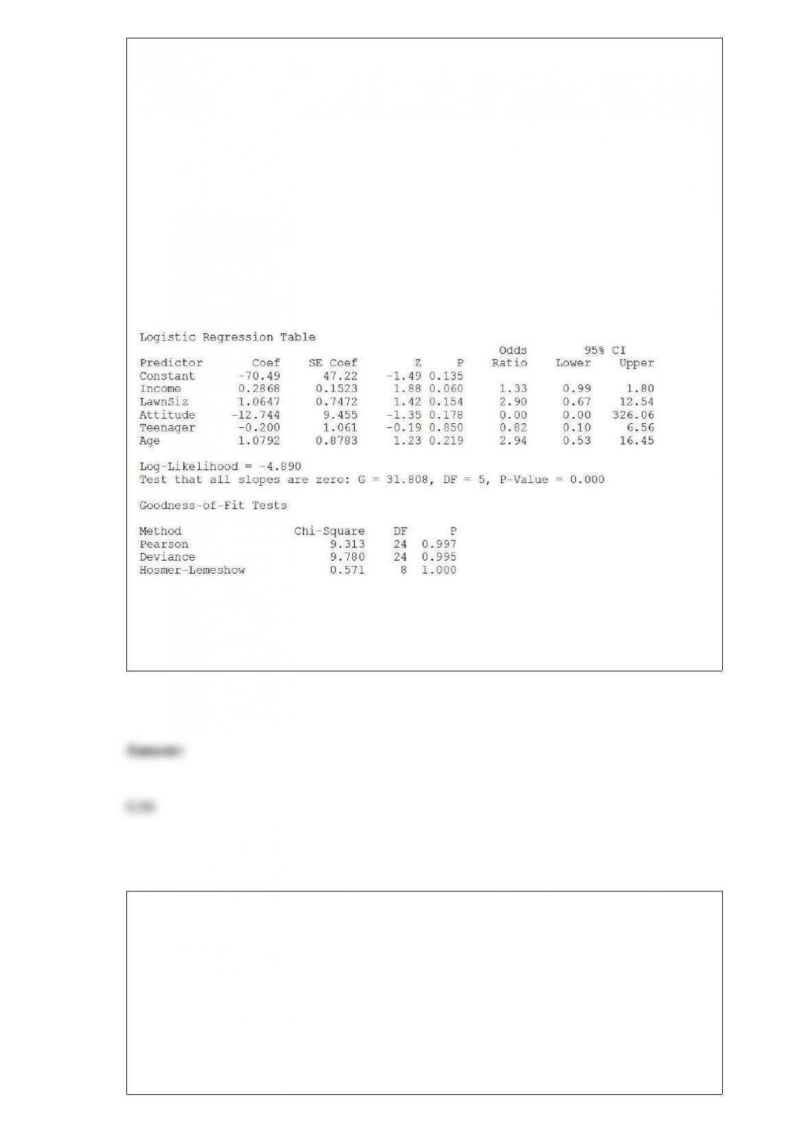
TABLE 17-12
The marketing manager for a nationally franchised lawn service company would like to
study the characteristics that differentiate home owners who do and do not have a lawn
service. A random sample of 30 home owners located in a suburban area near a large
city was selected; 15 did not have a lawn service (code 0) and 15 had a lawn service
(code 1). Additional information available concerning these 30 home owners includes
family income (Income, in thousands of dollars), lawn size (Lawn Size, in thousands of
square feet), attitude toward outdoor recreational activities (Attitude 0 = unfavorable, 1
= favorable), number of teenagers in the household (Teenager), and age of the head of
the household (Age).
The Minitab output is given below:
Referring to Table 17-12, what is the p-value of the test statistic when testing whether
Income makes a significant contribution to the model in the presence of the other
independent variables?
TABLE 15-6
Given below are results from the regression analysis on 40 observations where the
dependent variable is the number of weeks a worker is unemployed due to a layoff (Y)
and the independent variables are the age of the worker (X1), the number of years of
education received (X2), the number of years at the previous job (X3), a dummy variable
for marital status (X4: 1 = married, 0 = otherwise), a dummy variable for head of
household (X5: 1 = yes, 0 = no) and a dummy variable for management position (X6: 1
= yes, 0 = no).
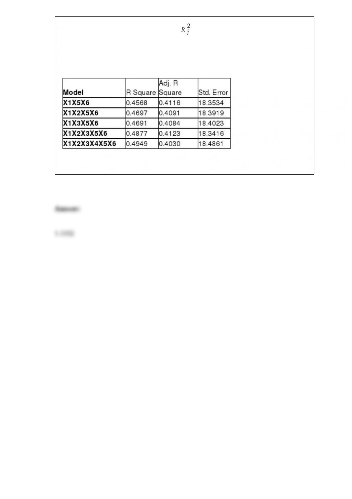
The coefficient of multiple determination ( ) for the regression model using each of
the 6 variables Xj as the dependent variable and all other X variables as independent
variables are, respectively, 0.2628, 0.1240, 0.2404, 0.3510, 0.3342 and 0.0993.
The partial results from best-subset regression are given below:
Referring to Table 15-6, what is the value of the variance inflationary factor of
Manager?