115)
A southeastern college has an enrollment of 2951 female students. Records show that the mean
height of these students is 64.7 inches and that the standard deviation is 2.3 inches. The table shows
frequency and relative–frequency data for these heights. If you assume that the distribution of
heights is approximately normal, then you can use the table to estimate areas under the associated
normal curve (that is, under the normal curve that has parameters µ = 64.7 and = 2.3). Making
this assumption, estimate the area under the associated normal curve to the right of 63.
Height
(inches)
Freq. Relative
freq.
56–under 57 20.0007
57–under 58 70.0024
58–under 59 14 0.0047
59–under 60 31 0.0105
60–under 61 101 0.0342
61–under 62 194 0.0657
62–under 63 311 0.1054
63–under 64 410 0.1389
64–under 65 526 0.1782
65–under 66 482 0.1633
66–under 67 397 0.1345
67–under 68 254 0.0861
68–under 69 150 0.0508
69–under 70 49 0.0166
70–under 71 17 0.0058
71–under 72 50.0017
72–under 73 10.0003
115)
A)
0.2443
B)
0.2236
C)
0.1054
D)
0.7762
38
116)
Frequency data were reported for the ages of women who became mothers during one year in a
selected U.S. city. The age distribution is given in the table. Obtain a relative–frequency histogram
of these data and determine whether the ages are approximately normally distributed.
Age
(yrs)
Frequency
10–under 15 16
15–under 20 134
20–under 25 534
25–under 30 1043
30–under 35 982
35–under 40 399
40–under 45 94
45–under 50 7
116)
A)
Yes. The distribution is bell–shaped.
B)
No. The distribution is right–skewed.
C)
No. The distribution is left–skewed.
D)
No. The distribution is J–shaped.
Provide an appropriate response.
117)
True or false, areas under the standard normal curve cannot be negative, whereas z–scores can be
positive or negative.
117)
A)
True
B)
False
Estimate the indicated probability by using the normal distribution as an approximation to the binomial distribution.
118)
Two percent of hair dryers produced at a certain plant are defective. Estimate the probability that
of 10,000 randomly selected hair dryers, the number of defectives is between 195 and 210 inclusive.
118)
A)
0.4251
B)
0.4034
C)
0.4017
D)
0.3989
Provide an appropriate response. Assume that the variable under consideration has a density curve.
119)
The area under the density curve that lies between 29 and 46 is 0.456. What percentage of all
possible observations of the variable are either less than 29 or greater than 46?
119)
A)
29.4%
B)
54.4%
C)
45.6%
D)
70.6%
Find the indicated probability or percentage for the normally distributed variable.
120)
A bank‘s loan officer rates applicants for credit. The ratings are normally distributed with a mean of
200 and a standard deviation of 50. If an applicant is randomly selected, find the probability of a
rating that is between 170 and 220.
120)
A)
0.3811
B)
0.0703
C)
0.1554
D)
0.2257
Find the specified percentile, quartile, or decile.
121)
The weights of certain machine components are normally distributed with a mean of 8.53 g and a
standard deviation of 0.1 g. Find the 97th percentile.
121)
A)
8.55 g
B)
8.58 g
C)
8.80 g
D)
8.72 g
Use a table of areas for the standard normal curve to find the required z–score.
122)
Find the z–score for having area 0.07 to its right under the standard normal curve, that is, find
z0.07 .
122)
A)
1.39
B)
1.48
C)
1.26
D)
1.45
Fill in the blanks by standardizing the normally distributed variable.
123)
Dave drives to work each morning at about the same time. His commute time is normally
distributed with a mean of 45 minutes and a standard deviation of 5 minutes. The percentage of
time that his commute time exceeds 55 minutes is equal to the area under the standard normal
curve that lies to the ___ of ___.
123)
A)
left, 2
B)
left, 1.1
C)
right, 2
D)
right, 10
40
Use the empirical rule to solve the problem.
124)
The annual precipitation for one city is normally distributed with a mean of 347 inches and a
standard deviation of 3.3 inches. Fill in the blanks.
In 95.44% of the years, the precipitation in this city is between ___ and ___ inches.
124)
A)
337.1, 347
B)
347, 353.6
C)
337.1, 356.9
D)
340.4, 353.6
D)
Use a table of areas to find the specified area under the standard normal curve.
125)
The area that lies between –1.10 and –0.36
125)
A)
0.2239
B)
0.4951
C)
–0.2237
D)
0.2237
D)
Find the indicated probability or percentage for the normally distributed variable.
126)
A bank‘s loan officer rates applicants for credit. The ratings are normally distributed with a mean of
200 and a standard deviation of 50. If an applicant is randomly selected, find the probability of a
rating that is between 200 and 275.
126)
A)
0.4332
B)
0.9332
C)
0.0668
D)
0.5
D)
Estimate the indicated probability by using the normal distribution as an approximation to the binomial distribution.
127)
Two percent of hair dryers produced in a certain plant are defective. Estimate the probability that
of 10,000 randomly selected hair dryers, exactly 225 are defective.
127)
A)
0.0065
B)
0.0034
C)
0.0051
D)
0.0057
D)
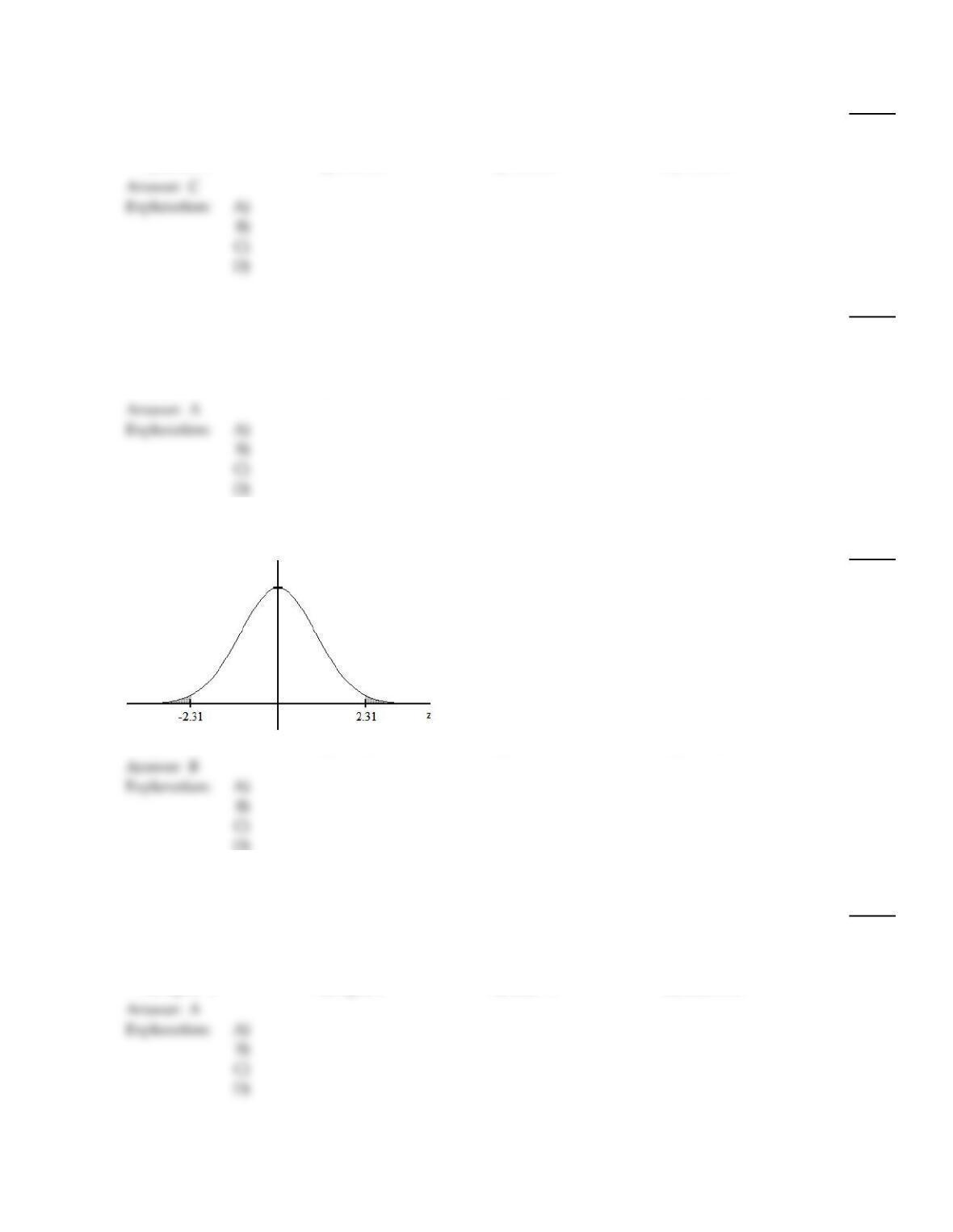
Use the empirical rule to solve the problem.
128)
The systolic blood pressure of 18–year–old women is normally distributed with a mean of 120
mmHg and a standard deviation of 12 mmHg. What percentage of 18–year–old women have a
systolic blood pressure between 96 mmHg and 144 mmHg?
128)
A)
68.26%
B)
99.74%
C)
95.44%
D)
99.99%
129)
The amount of Jen’s monthly phone bill is normally distributed with a mean of $66 and a standard
deviation of $8. Fill in the blanks.
68.26% of her phone bills are between $___ and $___.
129)
A)
58, 74
B)
50, 66
C)
50, 82
D)
66, 74
D)
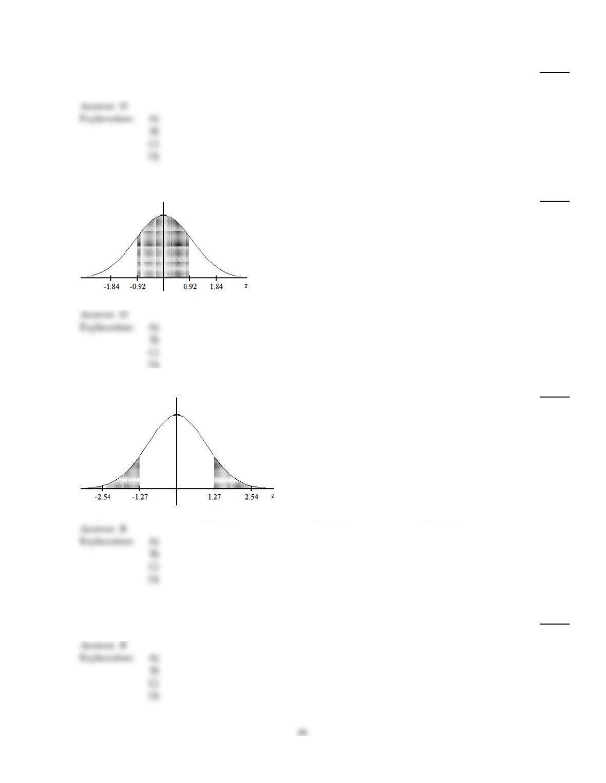
Use a table of areas to obtain the shaded area under the standard normal curve.
130)
130)
A)
0.9792
B)
0.0208
C)
0.0104
D)
0.9896
D)
Fill in the blanks by standardizing the normally distributed variable.
131)
The amount of time that customers wait in line during peak hours at one bank is normally
distributed with a mean of 13 minutes and a standard deviation of 3 minutes. The percentage of
time that the waiting time exceeds 10 minutes is equal to the area under the standard normal curve
that lies to the ___ of ___.
131)
A)
right, –1
B)
right, 1
C)
left, –1
D)
left, 0.54
42
D)
Provide an appropriate response.
132)
True or false, the mean of a normally distributed variable can be any real number.
132)
A)
True
B)
False
Use a table of areas for the standard normal curve to find the required z–score.
133)
Find the z–score for which the area under the standard normal curve to its left is 0.96
133)
A)
1.82
B)
1.75
C)
–1.38
D)
1.03
Find the indicated probability or percentage for the normally distributed variable.
134)
The variable X is normally distributed. The mean is µ= 15.2 and the standard deviation is = 0.9.
Find P(X > 16.1).
134)
A)
0.1550
B)
0.1357
C)
0.1587
D)
0.8413
Solve the problem.
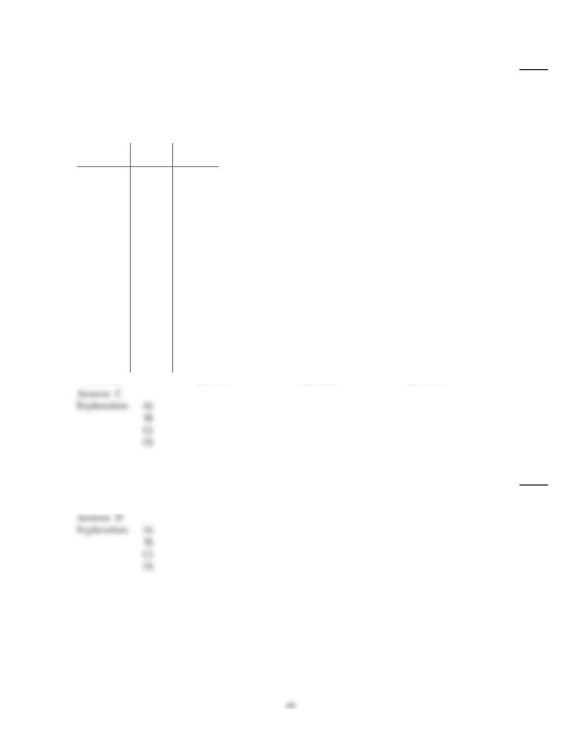
135)
A northeastern college has an enrollment of 2835 female students. Records show that the mean
height of these students is 65.2 inches and that the standard deviation is 2.8 inches. The table shows
frequency and relative–frequency data for these heights. If you assume that the distribution of
heights is approximately normal, then you can use the table to estimate areas under the associated
normal curve (that is, under the normal curve that has parameters µ = 65.2 and = 2.8). Making
this assumption, estimate the area under the associated normal curve between 65 and 70.
Height
(inches)
Freq. Relative
freq.
57–under 58 16 0.0056
58–under 59 25 0.0088
59–under 60 56 0.0198
60–under 61 96 0.0339
61–under 62 178 0.0628
62–under 63 263 0.0928
63–under 64 322 0.1136
64–under 65 388 0.1369
65–under 66 406 0.1432
66–under 67 361 0.1273
67–under 68 292 0.1030
68–under 69 201 0.0709
69–under 70 113 0.0399
70–under 71 75 0.0265
71–under 72 25 0.0088
72–under 73 16 0.0056
73–under 74 20.0007
135)
A)
0.1831
B)
0.5108
C)
0.4843
D)
0.6212
Use a table of areas for the standard normal curve to find the required z–score.
136)
Determine the two z–scores that divide the area under the standard normal curve into a middle
0.874 area and two outside 0.063 areas.
136)
A)
–1.45, 1.45
B)
–1.46, 1.46
C)
–1.39, 1.39
D)
–1.53, 1.53
Provide an appropriate response.
137)
Which of the following statements concerning the standard normal curve is/are true (if any)?
a. The area under the standard normal curve to the left of –3 is zero.
b. The area under the standard normal curve between any two z–scores is greater than zero.
c. The area under the standard normal curve between two z–scores will be negative if both z–scores
are negative.
d. The area under the standard normal curve to the left of any z–score is less than 1.
137)
A)
a, b
B)
b, d
C)
a
D)
a, c
Fill in the blanks by standardizing the normally distributed variable.
138)
Dave drives to work each morning at about the same time. His commute time is normally
distributed with a mean of 45 minutes and a standard deviation of 5 minutes. The percentage of
time that his commute time is less than 49 minutes is equal to the area under the standard normal
curve that lies to the ___ of __.
138)
A)
right, 1
B)
left, –0.8
C)
right, 0.8
D)
left, 0.8
Use a table of areas for the standard normal curve to find the required z–score.
139)
Find the z–score having area 0.09 to its left under the standard normal curve.
139)
A)
–1.26
B)
–1.45
C)
–1.39
D)
–1.34
140)
Find the z–score having area 0.86 to its right under the standard normal curve; that is, find z0.86 .
140)
A)
0.8051
B)
–1.08
C)
1.08
D)
0.5557
Find the indicated probability or percentage for the normally distributed variable.
141)
The lengths of human pregnancies are normally distributed with a mean of 268 days and a
standard deviation of 15 days. What is the probability that a pregnancy lasts at least 300 days?
141)
A)
0.0179
B)
0.4834
C)
0.9834
D)
0.0166
Use a table of areas to obtain the shaded area under the standard normal curve.
142)
142)
A)
0.1788
B)
0.8212
C)
0.3576
D)
0.6424
143)
143)
A)
0.7960
B)
0.2040
C)
0.1020
D)
0.8980
Use a table of areas to find the specified area under the standard normal curve.
144)
The area that lies between –0.73 and 2.27
144)
A)
0.4884
B)
0.7557
C)
0.2211
D)
1.54
Answer Key
Testname: C6
Answer Key
Testname: C6
48
Answer Key
Testname: C6
49
Answer Key
Testname: C6
50
Answer Key
Testname: C6
Answer Key
Testname: C6
Answer Key
Testname: C6