
Chapter 3 – Linear Programming: Sensitivity Analysis and Interpretation of Solution
TOPICS:
Interpretation of Management Scientist output
50. LINDO output is given for the following linear programming problem.
MIN 12 X1 + 10 X2 + 9 X3
SUBJECT TO
2) 5 X1 + 8 X2 + 5 X3 >= 60
3) 8 X1 + 10 X2 + 5 X3 >= 80
END
LP OPTIMUM FOUND AT STEP 1
OBJECTIVE FUNCTION VALUE
1) 80.000000
VARIABLE
VALUE
REDUCED COST
X1
.000000
4.000000
X2
8.000000
.000000
X3
.000000
4.000000
ROW
SLACK OR SURPLUS
DUAL PRICE
2)
4.000000
.000000
3)
.000000
−1.000000
NO. ITERATIONS= 1
RANGES IN WHICH THE BASIS IS UNCHANGED:
OBJ. COEFFICIENT RANGES
VARIABLE
CURRENT
COEFFICIENT
ALLOWABLE
INCREASE
ALLOWABLE
DECREASE
X1
12.000000
INFINITY
4.000000
X2
10.000000
5.000000
10.000000
X3
9.000000
INFINITY
4.000000
RIGHTHAND SIDE RANGES
ROW
CURRENT
RHS
ALLOWABLE
INCREASE
ALLOWABLE
DECREASE
2
60.000000
4.000000
INFINITY
3
80.000000
INFINITY
5.000000
a.
What is the solution to the problem?
b.
Which constraints are binding?
c.
Interpret the reduced cost for x1.
d.
Interpret the dual price for constraint 2.
e.
What would happen if the cost of x1 dropped to 10 and the cost of x2 increased to 12?
b.
Constraint 2 is binding.
d.
Increasing the right-hand side by 1 will cause a negative improvement, or increase, of 1 in

Chapter 3 – Linear Programming: Sensitivity Analysis and Interpretation of Solution
51. The LP problem whose output follows determines how many necklaces, bracelets, rings, and earrings a jewelry store
should stock. The objective function measures profit; it is assumed that every piece stocked will be sold. Constraint 1
measures display space in units, constraint 2 measures time to set up the display in minutes. Constraints 3 and 4 are
marketing restrictions.
LINEAR PROGRAMMING PROBLEM
MAX 100X1+120X2+150X3+125X4
S.T.
1) X1+2X2+2X3+2X4<108
2) 3X1+5X2+X4<120
3) X1+X3<25
4) X2+X3+X4>50
OPTIMAL SOLUTION
Objective Function Value = 7475.000
Variable
Value
Reduced Cost
X1
8.000
0.000
X2
0.000
5.000
X3
17.000
0.000
X4
33.000
0.000
Constraint
Slack/Surplus
Dual Price
1
0.000
75.000
2
63.000
0.000
3
0.000
25.000
4
0.000
−25.000
OBJECTIVE COEFFICIENT RANGES
Variable
Lower Limit
Current Value
Upper Limit
X1
87.500
100.000
No Upper Limit
X2
No Lower Limit
120.000
125.000
X3
125.000
150.000
162.500
X4
120.000
125.000
150.000
RIGHT HAND SIDE RANGES
Constraint
Lower Limit
Current Value
Upper Limit
1
100.000
108.000
123.750
2
57.000
120.000
No Upper Limit
3
8.000
25.000
58.000
4
41.500
50.000
54.000
Use the output to answer the questions.
a.
How many necklaces should be stocked?
this minimization objective function.
e.
The sum of the percentage changes is (−2)/(−4) + 2/5 < 1 so the solution would not change.
1
Interpretation of LINDO output
Chapter 3 – Linear Programming: Sensitivity Analysis and Interpretation of Solution
b.
Now many bracelets should be stocked?
c.
How many rings should be stocked?
d.
How many earrings should be stocked?
e.
How much space will be left unused?
f.
How much time will be used?
g.
By how much will the second marketing restriction be exceeded?
h.
What is the profit?
i.
To what value can the profit on necklaces drop before the solution would change?
j.
By how much can the profit on rings increase before the solution would change?
k.
By how much can the amount of space decrease before there is a change in the profit?
l.
You are offered the chance to obtain more space. The offer is for 15 units and the total price
is 1500. What should you do?
a.
b.
c.
17
d.
33
e.
f.
57
g.
h.
7475
i.
k.
l.
Say no. Although 15 units can be evaluated, their value (1125) is less than the cost (1500).
Interpretation of Management Scientist output
52. The decision variables represent the amounts of ingredients 1, 2, and 3 to put into a blend. The objective function
represents profit. The first three constraints measure the usage and availability of resources A, B, and C. The fourth
constraint is a minimum requirement for ingredient 3. Use the output to answer these questions.
a.
How much of ingredient 1 will be put into the blend?
b.
How much of ingredient 2 will be put into the blend?
c.
How much of ingredient 3 will be put into the blend?
d.
How much resource A is used?
e.
How much resource B will be left unused?
f.
What will the profit be?
g.
What will happen to the solution if the profit from ingredient 2 drops to 4?
h.
What will happen to the solution if the profit from ingredient 3 increases by 1?
i.
What will happen to the solution if the amount of resource C increases by 2?
j.
What will happen to the solution if the minimum requirement for ingredient 3 increases to
15?
LINEAR PROGRAMMING PROBLEM
MAX 4X1+6X2+7X3
S.T.
1) 3X1+2X2+5X3<120
2) 1X1+3X2+3X3<80
3) 5X1+5X2+8X3<160
4) +1X3>10
Chapter 3 – Linear Programming: Sensitivity Analysis and Interpretation of Solution
OPTIMAL SOLUTION
Objective Function Value = 166.000
Variable
Value
Reduced Cost
X1
0.000
2.000
X2
16.000
0.000
X3
10.000
0.000
Constraint
Slack/Surplus
Dual Price
1
38.000
0.000
2
2.000
0.000
3
0.000
1.200
4
0.000
−2.600
OBJECTIVE COEFFICIENT RANGES
Variable
Lower Limit
Current Value
Upper Limit
X1
No Lower Limit
4.000
6.000
X2
4.375
6.000
No Upper Limit
X3
No Lower Limit
7.000
9.600
RIGHT HAND SIDE RANGES
Constraint
Lower Limit
Current Value
Upper Limit
1
82.000
120.000
No Upper Limit
2
78.000
80.000
No Upper Limit
3
80.000
160.000
163.333
4
8.889
10.000
20.000
0
b.
16
10
d.
44
2
166
g.
rerun
h.
Z = 176
Z = 168.4
Z = 153
1
Interpretation of Management Scientist output
53. The LP model and LINDO output represent a problem whose solution will tell a specialty retailer how many of four
different styles of umbrellas to stock in order to maximize profit. It is assumed that every one stocked will be sold. The
variables measure the number of women’s, golf, men’s, and folding umbrellas, respectively. The constraints measure
storage space in units, special display racks, demand, and a marketing restriction, respectively.
MAX 4 X1 + 6 X2 + 5 X3 + 3.5 X4
SUBJECT TO
2) 2 X1 + 3 X2 + 3 X3 + X4 <= 120
3) 1.5 X1 + 2 X2 <= 54
4) 2 X2 + X3 + X4 <= 72

Chapter 3 – Linear Programming: Sensitivity Analysis and Interpretation of Solution
5) X2 + X3 >= 12
END
OBJECTIVE FUNCTION VALUE
1) 318.00000
VARIABLE
VALUE
REDUCED COST
X1
12.000000
.000000
X2
.000000
.500000
X3
12.000000
.000000
X4
60.000000
.000000
ROW
SLACK OR SURPLUS
DUAL PRICE
2)
.000000
2.000000
3)
36.000000
.000000
4)
.000000
1.500000
5)
.000000
−2.500000
RANGES IN WHICH THE BASIS IS UNCHANGED:
OBJ. COEFFICIENT RANGES
VARIABLE
CURRENT
COEFFICIENT
ALLOWABLE
INCREASE
ALLOWABLE
DECREASE
X1
4.000000
1.000000
2.500000
X2
6.000000
.500000
INFINITY
X3
5.000000
2.500000
.500000
X4
3.500000
INFINITY
.500000
RIGHTHAND SIDE RANGES
ROW
CURRENT
RHS
ALLOWABLE
INCREASE
ALLOWABLE
DECREASE
2
120.000000
48.000000
24.000000
3
54.000000
INFINITY
36.000000
4
72.000000
24.000000
48.000000
5
12.000000
12.000000
12.000000
Use the output to answer the questions.
a.
How many women’s umbrellas should be stocked?
b.
How many golf umbrellas should be stocked?
c.
How many men’s umbrellas should be stocked?
d.
How many folding umbrellas should be stocked?
e.
How much space is left unused?
f.
How many racks are used?
g.
By how much is the marketing restriction exceeded?
h.
What is the total profit?
i.
By how much can the profit on women’s umbrellas increase before the solution would
change?
j.
To what value can the profit on golf umbrellas increase before the solution would change?
k.
By how much can the amount of space increase before there is a change in the dual price?
l.
You are offered an advertisement that should increase the demand constraint from 72 to 86
for a total cost of $20. Would you say yes or no?
a.
12

Chapter 3 – Linear Programming: Sensitivity Analysis and Interpretation of Solution
54. Eight of the entries have been deleted from the LINDO output that follows. Use what you know about linear
programming to find values for the blanks.
MIN 6 X1 + 7.5 X2 + 10 X3
SUBJECT TO
2) 25 X1 + 35 X2 + 30 X3 >= 2400
3) 2 X1 + 4 X2 + 8 X3 >= 400
END
LP OPTIMUM FOUND AT STEP 2
OBJECTIVE FUNCTION VALUE
1) 612.50000
VARIABLE
VALUE
REDUCED COST
X1
________
1.312500
X2
________
________
X3
27.500000
________
ROW
SLACK OR SURPLUS
DUAL PRICE
2)
________
−.125000
3)
________
−.781250
NO. ITERATIONS= 2
RANGES IN WHICH THE BASIS IS UNCHANGED:
OBJ. COEFFICIENT RANGES
VARIABLE
CURRENT
COEFFICIENT
ALLOWABLE
INCREASE
ALLOWABLE
DECREASE
X1
6.000000
_________
_________
X2
7.500000
1.500000
2.500000
X3
10.000000
5.000000
3.571429
RIGHTHAND SIDE RANGES
ROW
CURRENT
ALLOWABLE
ALLOWABLE
b.
12
d.
60
18
g.
h.
318
6.5
k.
48
Interpretation of solution

Chapter 3 – Linear Programming: Sensitivity Analysis and Interpretation of Solution
RHS
INCREASE
DECREASE
2
2400.000000
1100.000000
900.000000
3
400.000000
240.000000
125.714300
1
Interpretation of solution
55. Portions of a Management Scientist output are shown below. Use what you know about the solution of linear
programs to fill in the ten blanks.
LINEAR PROGRAMMING PROBLEM
MAX 12X1+9X2+7X3
S.T.
1) 3X1+5X2+4X3<150
2) 2X1+1X2+1X3<64
3) 1X1+2X2+1X3<80
4) 2X1+4X2+3X3>116
OPTIMAL SOLUTION
Objective Function Value = 336.000
Variable
Value
Reduced Cost
X1
______
0.000
X2
24.000
______
X3
______
3.500
Constraint
Slack/Surplus
Dual Price
1
0.000
15.000
2
______
0.000
3
______
0.000
4
0.000
______
OBJECTIVE COEFFICIENT RANGES
Variable
Lower Limit
Current Value
Upper Limit
X1
5.400
12.000
No Upper Limit
X2
2.000
9.000
20.000
X3
No Lower Limit
7.000
10.500
RIGHT HAND SIDE RANGES
Constraint
Lower Limit
Current Value
Upper Limit
1
145.000
150.000
156.667
2
______
______
64.000
3
______
______
80.000
4
110.286
116.000
120.000
Chapter 3 – Linear Programming: Sensitivity Analysis and Interpretation of Solution
Interpretation of solution
56. A large sporting goods store is placing an order for bicycles with its supplier. Four models can be ordered: the adult
Open Trail, the adult Cityscape, the girl’s Sea Sprite, and the boy’s Trail Blazer. It is assumed that every bike ordered will
be sold, and their profits, respectively, are 30, 25, 22, and 20. The LP model should maximize profit. There are several
conditions that the store needs to worry about. One of these is space to hold the inventory. An adult’s bike needs two feet,
but a child’s bike needs only one foot. The store has 500 feet of space. There are 1200 hours of assembly time available.
The child’s bike need 4 hours of assembly time; the Open Trail needs 5 hours and the Cityscape needs 6 hours. The store
would like to place an order for at least 275 bikes.
a.
Formulate a model for this problem.
b.
Solve your model with any computer package available to you.
c.
How many of each kind of bike should be ordered and what will the profit be?
d.
What would the profit be if the store had 100 more feet of storage space?
e.
If the profit on the Cityscape increases to $35, will any of the Cityscape bikes be ordered?
f.
Over what range of assembly hours is the dual price applicable?
g.
If we require 5 more bikes in inventory, what will happen to the value of the optimal
solution?
h.
Which resource should the company work to increase, inventory space or assembly time?
a.
MAX 30 X1 + 25 X2 + 22 X3 + 20 X4
SUBJECT TO
2) 2 X1 + 2 X2 + X3 + X4 <= 500
3) 5 X1 + 6 X2 + 4 X3 + 4 X4 <= 1200
4) X1 + X2 + X3 + X4 >= 275
b.
OBJECTIVE FUNCTION VALUE
1) 6850.0000
VARIABLE
VALUE
REDUCED COST
100.000000
13.000000
175.000000
SLACK OR SURPLUS
2)
125.000000
3)
4)
RANGES IN WHICH THE BASIS IS UNCHANGED:
Chapter 3 – Linear Programming: Sensitivity Analysis and Interpretation of Solution
OBJ. COEFFICIENT RANGES
CURRENT
COEFFICIENT
ALLOWABLE
INCREASE
ALLOWABLE
DECREASE
X1
30.000000
INFINITY
2.500000
X2
25.000000
13.000000
INFINITY
X3
22.000000
2.000000
2.000000
X4
20.000000
2.000000
INFINITY
RIGHTHAND SIDE RANGES
INCREASE
DECREASE
500.000000
INFINITY
125.000000
1200.000000
125.000000
100.000000
275.000000
25.000000
35.000000
Order 100 Open Trails, 0 Cityscapes, 175 Sea Sprites, and 0 Trail Blazers. Profit will be
d.
6850
No. The $10 increase is below the reduced cost.
1100 to 1325
g.
h.
Assembly time.
1
Formulation and computer solution
57. A company produces two products made from aluminum and copper. The table below gives the unit requirements, the
unit production man–hours required, the unit profit and the availability of the resources (in tons).
Aluminum
Copper
Man-hours
Unit Profit
Product 1
1
0
2
50
Product 2
1
1
3
60
Available
10
6
24
The Management Scientist provided the following solution output:
Objective Function Value = 540.000
VARIABLE
VALUE
REDUCED COST
X1
6.000
0.000
X2
4.000
0.000
CONSTRAINT
SLACK/SURPLUS
DUAL PRICE
1
.000
30.000
2
2.000
0.000
3
0.000
10.000
RANGES IN WHICH THE BASIS IS UNCHANGED:
OBJ. COEFFICIENT RANGES
VARIABLE
CURRENT
COEFFICIENT
ALLOWABLE
INCREASE
ALLOWABLE
DECREASE
X1
50.000
10.000
10.000
X2
60.000
15.000
10.000
RIGHTHAND SIDE RANGES
Chapter 3 – Linear Programming: Sensitivity Analysis and Interpretation of Solution
CONSTRAINT
CURRENT
RHS
ALLOWABLE
INCREASE
ALLOWABLE
DECREASE
1
10.000
2.000
1.000
2
6.000
INFINITY
2.000
3
24.000
2.000
4.000
a.
What is the optimal production schedule?
b.
Within what range for the profit on product 2 will the solution in (a) remain optimal? What is
the optimal profit when c2 = 70?
c.
Suppose that simultaneously the unit profits on x1 and x2 changed from 50 to 55 and 60 to 65
respectively. Would the optimal solution change?
d.
Explain the meaning of the “DUAL PRICES” column. Given the optimal solution, why
should the dual price for copper be 0?
e.
What is the increase in the value of the objective function for an extra unit of aluminum?
f.
Man-hours were not figured into the unit profit as it must pay three workers for eight hours
of work regardless of the number of man-hours used. What is the dual price for man-hours?
Interpret.
g.
On the other hand, aluminum and copper are resources that are ordered as needed. The unit
profit coefficients were determined by: (selling price per unit) – (cost of the resources per
unit). The 10 units of aluminum cost the company $100. What is the most the company
should be willing to pay for extra aluminum?
a.
6 product 1, 4 product 2, Profit = $540
Between $50 and $75; at $70 the profit is $580
c.
No; total % change is 83 1/3% < 100%
d.
The shadow price is the “premium” for aluminum — would be willing to pay up to $10 + $30
1
Interpretation of solution
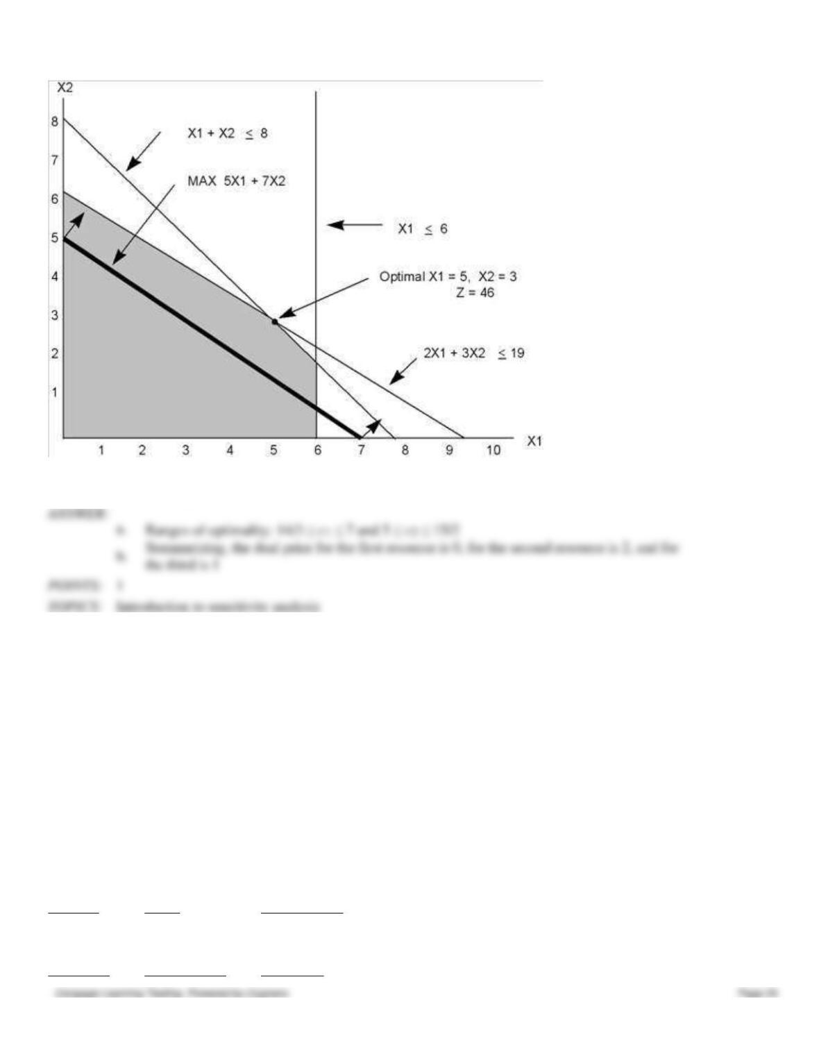
58. Given the following linear program:
MAX
5x1 + 7x2
s.t.
x1 ≤ 6
2x1 + 3x2 ≤ 19
x1 + x2 ≤ 8
x1, x2 ≥ 0
The graphical solution to the problem is shown below. From the graph we see that the optimal solution occurs at x1 = 5, x2
= 3, and z = 46.
Chapter 3 – Linear Programming: Sensitivity Analysis and Interpretation of Solution
a.
Calculate the range of optimality for each objective function coefficient.
b.
Calculate the dual price for each resource.
Introduction to sensitivity analysis
59. Consider the following linear program:
MAX
3x1 + 4x2 ($ Profit)
s.t.
x1 + 3x2 ≤ 12
2x1 + x 2 ≤ 8
x1 ≤ 3
x1, x2 ≥ 0
The Management Scientist provided the following solution output:
OPTIMAL SOLUTION
Objective Function Value = 20.000
Variable
Value
Reduced Cost
X1
2.400
0.000
X2
3.200
0.000
Constraint
Slack/Surplus
Dual Price

Chapter 3 – Linear Programming: Sensitivity Analysis and Interpretation of Solution
1
0.000
1.000
2
0.000
1.000
3
0.600
0.000
OBJECTIVE COEFFICIENT RANGES
Variable
Lower Limit
Current Value
Upper Limit
X1
1.333
3.000
8.000
X2
1.500
4.000
9.000
RIGHT HAND SIDE RANGES
Constraint
Lower Limit
Current Value
Upper Limit
1
9.000
12.000
24.000
2
4.000
8.000
9.000
3
2.400
3.000
No Upper Limit
a.
What is the optimal solution including the optimal value of the objective function?
b.
Suppose the profit on x1 is increased to $7. Is the above solution still optimal? What is the
value of the objective function when this unit profit is increased to $7?
c.
If the unit profit on x2 was $10 instead of $4, would the optimal solution change?
d.
If simultaneously the profit on x1 was raised to $5.5 and the profit on x2 was reduced to $3,
would the current solution still remain optimal?
a.
Optimal solution will not change. Optimal profit will equal $29.60.
c.
Because 10 is outside the range of 1.5 to 9.0, the optimal solution likely would change.
1
Interpretation of solution
60. Consider the following linear program:
MIN
6x1 + 9x2 ($ cost)
s.t.
x1 + 2x2 ≤ 8
10x1 + 7.5x2 ≥ 30
x2 ≥ 2
x1, x2 ≥ 0
The Management Scientist provided the following solution output:
OPTIMAL SOLUTION
Objective Function Value = 27.000
Variable
Value
Reduced Cost
X1
1.500
0.000
X2
2.000
0.000
Constraint
Slack/Surplus
Dual Price
1
2.500
0.000
Chapter 3 – Linear Programming: Sensitivity Analysis and Interpretation of Solution
2
0.000
−0.600
3
0.000
−4.500
OBJECTIVE COEFFICIENT RANGES
Variable
Lower Limit
Current Value
Upper Limit
X1
0.000
6.000
12.000
X2
4.500
9.000
No Upper Limit
RIGHT HAND SIDE RANGES
Constraint
Lower Limit
Current Value
Upper Limit
1
5.500
8.000
No Upper Limit
2
15.000
30.000
55.000
3
0.000
2.000
4.000
a.
What is the optimal solution including the optimal value of the objective function?
b.
Suppose the unit cost of x1 is decreased to $4. Is the above solution still optimal? What is the
value of the objective function when this unit cost is decreased to $4?
c.
How much can the unit cost of x2 be decreased without concern for the optimal solution
changing?
d.
If simultaneously the cost of x1 was raised to $7.5 and the cost of x2 was reduced to $6,
would the current solution still remain optimal?
e.
If the right-hand side of constraint 3 is increased by 1, what will be the effect on the optimal
solution?
will be $24.00.
would not change.
e.
1
Interpretation of solution
Essay
61. Describe each of the sections of output that come from The Management Scientist and how you would use each.
Answer not provided.
1
Interpretation of computer output
62. Explain the connection between reduced costs and the range of optimality, and between dual prices and the range of
feasibility.
Answer not provided.
1
Interpretation of computer output
63. Explain the two interpretations of dual prices based on the accounting assumptions made in calculating the objective
function coefficients.

Chapter 3 – Linear Programming: Sensitivity Analysis and Interpretation of Solution
64. How can the interpretation of dual prices help provide an economic justification for new technology?
65. How is sensitivity analysis used in linear programming? Given an example of what type of questions that can be
answered.
66. How would sensitivity analysis of a linear program be undertaken if one wishes to consider simultaneous changes for
both the right-hand-side values and objective function.