Chapter 2 – An Introduction to Linear Programming
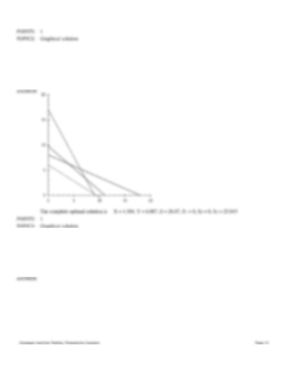
48. Find the complete optimal solution to this linear programming problem.
Max
2X + 3Y
s.t.
4X + 9Y ≤ 72
10X + 11Y ≤ 110
17X + 9Y ≤ 153
X , Y ≥ 0
49. Find the complete optimal solution to this linear programming problem.
Min
3X + 3Y
s.t.
12X + 4Y ≥ 48
10X + 5Y ≥ 50
4X + 8Y ≥ 32
X , Y ≥ 0
Chapter 2 – An Introduction to Linear Programming
Graphical solution
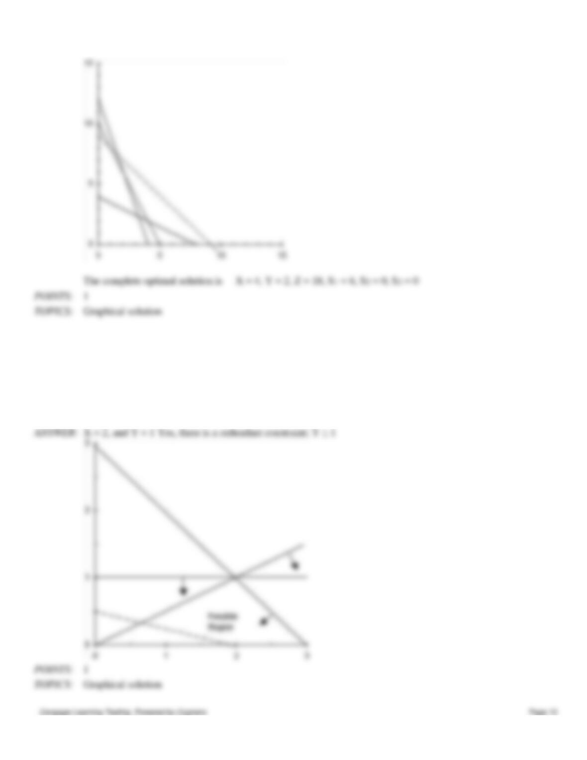
50. For the following linear programming problem, determine the optimal solution by the graphical solution method. Are
any of the constraints redundant? If yes, then identify the constraint that is redundant.
Max
X + 2Y
s.t.
X + Y ≤ 3
X − 2Y ≥ 0
Y ≤ 1
X, Y ≥ 0
Graphical solution
Chapter 2 – An Introduction to Linear Programming
51. Maxwell Manufacturing makes two models of felt tip marking pens. Requirements for each lot of pens are given
below.
Fliptop Model
Tiptop Model
Available
Plastic
3
4
36
Ink Assembly
5
4
40
Molding Time
5
2
30
The profit for either model is $1000 per lot.
a.
What is the linear programming model for this problem?
b.
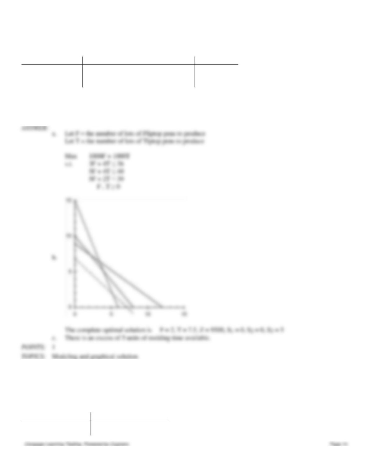
Find the optimal solution.
c.
Will there be excess capacity in any resource?
a.
Let F = the number of lots of Fliptop pens to produce
Let T = the number of lots of Tiptop pens to produce
Max
1000F + 1000T
s.t.
3F + 4T ≤ 36
5F + 4T ≤ 40
5F + 2T ≤ 30
c.
There is an excess of 5 units of molding time available.
Modeling and graphical solution
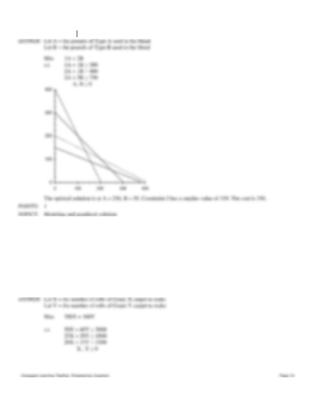
52. The Sanders Garden Shop mixes two types of grass seed into a blend. Each type of grass has been rated (per pound)
according to its shade tolerance, ability to stand up to traffic, and drought resistance, as shown in the table. Type A seed
costs $1 and Type B seed costs $2. If the blend needs to score at least 300 points for shade tolerance, 400 points for traffic
resistance, and 750 points for drought resistance, how many pounds of each seed should be in the blend? Which targets
will be exceeded? How much will the blend cost?
Type A
Type B
Shade Tolerance
1
1
Traffic Resistance
2
1
Chapter 2 – An Introduction to Linear Programming
Drought Resistance
2
5
Modeling and graphical solution
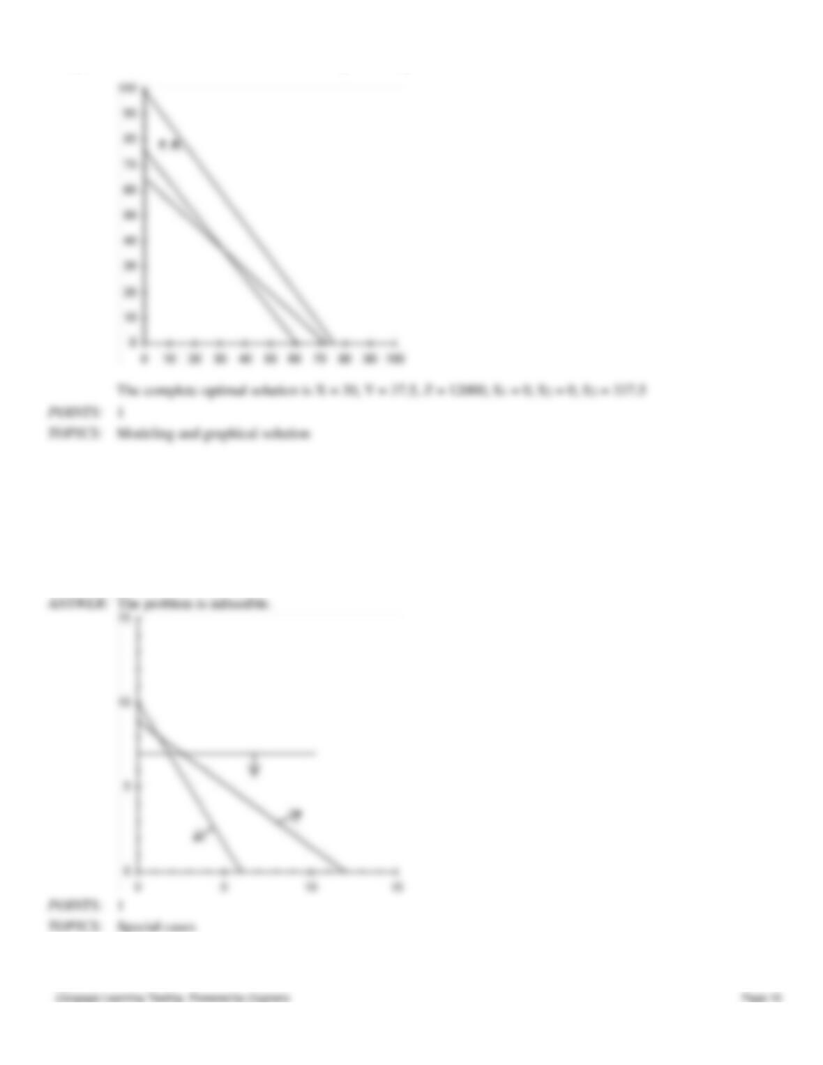
53. Muir Manufacturing produces two popular grades of commercial carpeting among its many other products. In the
coming production period, Muir needs to decide how many rolls of each grade should be produced in order to maximize
profit. Each roll of Grade X carpet uses 50 units of synthetic fiber, requires 25 hours of production time, and needs 20
units of foam backing. Each roll of Grade Y carpet uses 40 units of synthetic fiber, requires 28 hours of production time,
and needs 15 units of foam backing.
The profit per roll of Grade X carpet is $200 and the profit per roll of Grade Y carpet is $160. In the coming production
period, Muir has 3000 units of synthetic fiber available for use. Workers have been scheduled to provide at least 1800
hours of production time (overtime is a possibility). The company has 1500 units of foam backing available for use.
Develop and solve a linear programming model for this problem.
Chapter 2 – An Introduction to Linear Programming
54. Does the following linear programming problem exhibit infeasibility, unboundedness, or alternate optimal solutions?
Explain.
Min
1X + 1Y
s.t.
5X + 3Y ≤ 30
3X + 4Y ≥ 36
Y ≤ 7
X , Y ≥ 0
Special cases
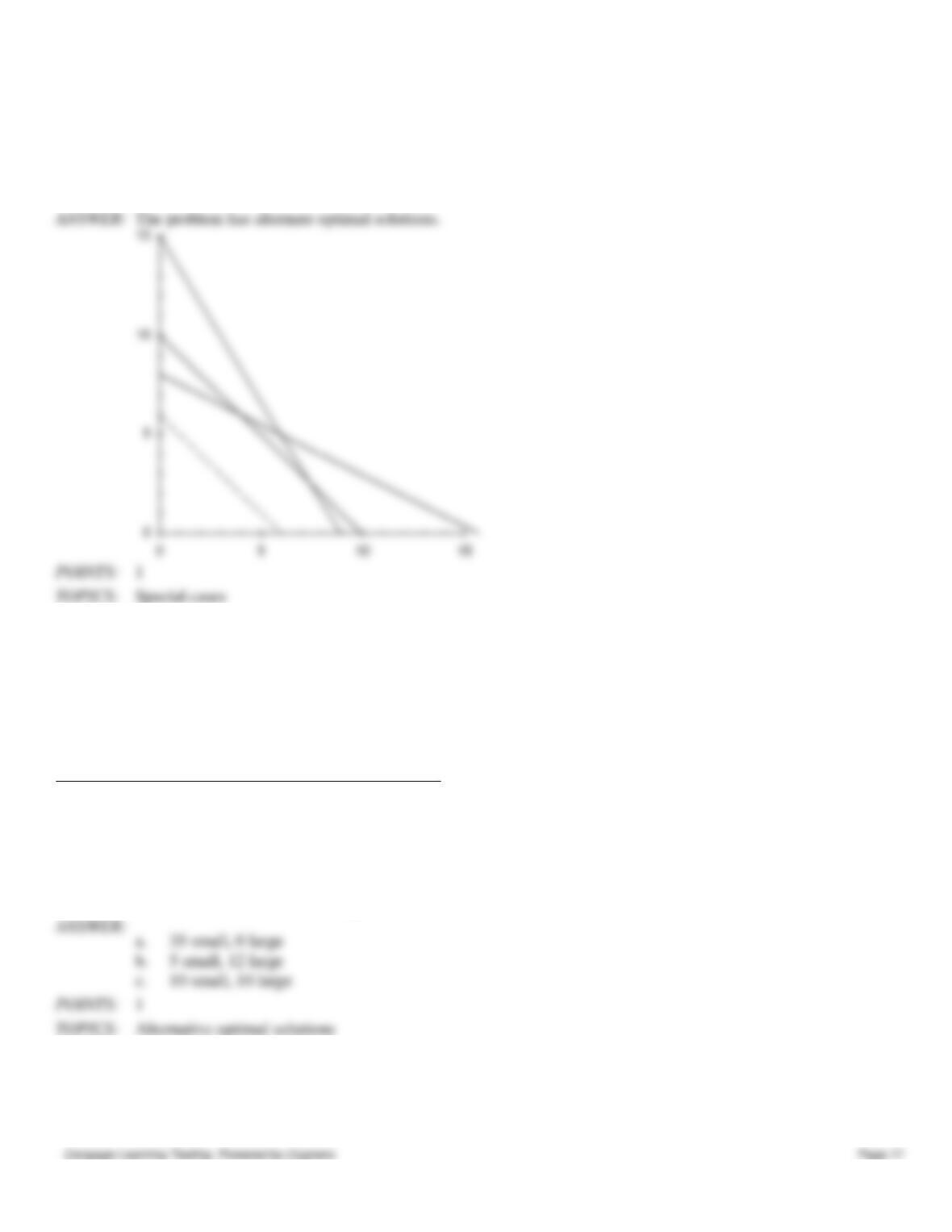
55. Does the following linear programming problem exhibit infeasibility, unboundedness, or alternate optimal solutions?
Explain.
Modeling and graphical solution
Chapter 2 – An Introduction to Linear Programming
Min
3X + 3Y
s.t.
1X + 2Y ≤ 16
1X + 1Y ≤ 10
5X + 3Y ≤ 45
X , Y ≥ 0
Special cases
56. A businessman is considering opening a small specialized trucking firm. To make the firm profitable, it is estimated
that it must have a daily trucking capacity of at least 84,000 cu. ft. Two types of trucks are appropriate for the specialized
operation. Their characteristics and costs are summarized in the table below. Note that truck 2 requires 3 drivers for long
haul trips. There are 41 potential drivers available and there are facilities for at most 40 trucks. The businessman’s
objective is to minimize the total cost outlay for trucks.
Capacity
Drivers
Truck
Cost
(Cu. Ft.)
Needed
Small
$18,000
2,400
1
Large
$45,000
6,000
3
Solve the problem graphically and note there are alternate optimal solutions. Which optimal solution:
a.
uses only one type of truck?
b.
utilizes the minimum total number of trucks?
c.
uses the same number of small and large trucks?
a.
35 small, 0 large
b.
5 small, 12 large
c.
10 small, 10 large
Alternative optimal solutions
57. Consider the following linear program:
Max
60X + 43Y
s.t.
X + 3Y ≥ 9
Chapter 2 – An Introduction to Linear Programming
6X − 2Y = 12
X + 2Y ≤ 10
X, Y ≥ 0
a.
Write the problem in standard form.
b.
What is the feasible region for the problem?
c.
Show that regardless of the values of the actual objective function coefficients, the optimal
solution will occur at one of two points. Solve for these points and then determine which one
maximizes the current objective function.
a.
Max
60X + 43Y
6X − 2Y = 12
b.
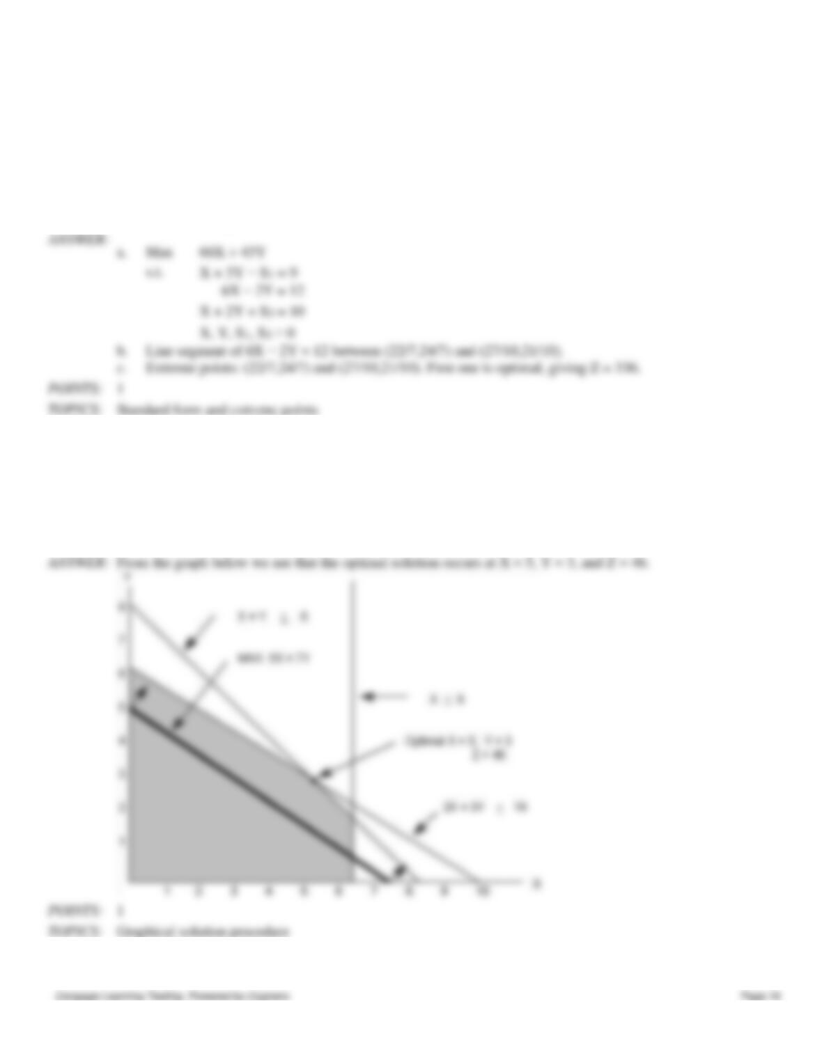
Line segment of 6X − 2Y = 12 between (22/7,24/7) and (27/10,21/10).
c.
Extreme points: (22/7,24/7) and (27/10,21/10). First one is optimal, giving Z = 336.
Standard form and extreme points
58. Solve the following linear program graphically.
Max
5X + 7Y
s.t.
X ≤ 6
2X + 3Y ≤ 19
X + Y ≤ 8
X, Y ≥ 0
Graphical solution procedure
59. Given the following linear program:
Chapter 2 – An Introduction to Linear Programming
Min
150X + 210Y
s.t.
3.8X + 1.2Y ≥ 22.8
Y ≥ 6
Y ≤ 15
45X + 30Y = 630
X, Y ≥ 0
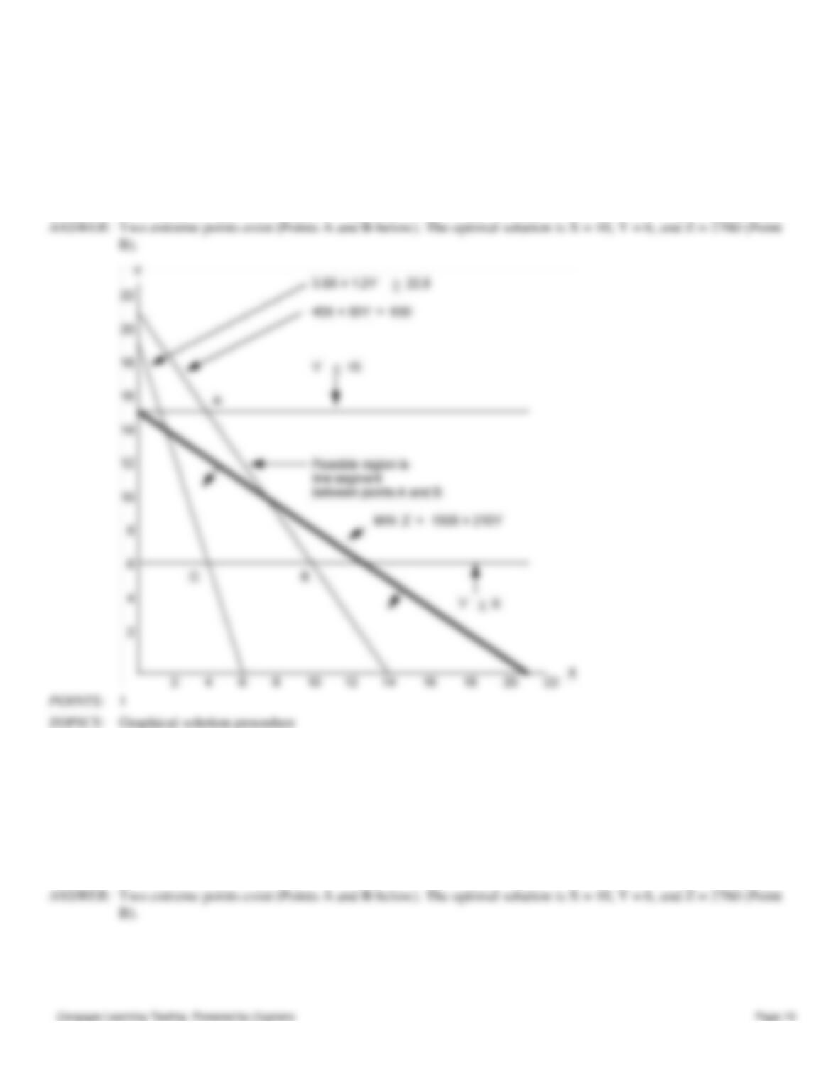
Solve the problem graphically. How many extreme points exist for this problem?
Graphical solution procedure
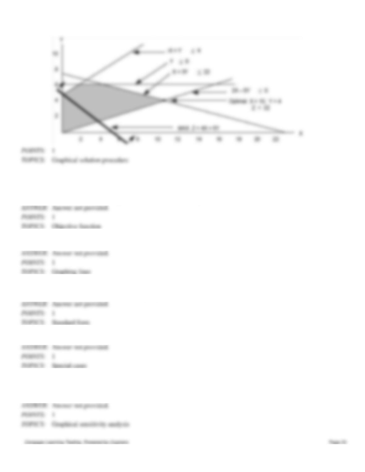
60. Solve the following linear program by the graphical method.
Max
4X + 5Y
s.t.
X + 3Y ≤ 22
−X + Y ≤ 4
Y ≤ 6
2X − 5Y ≤ 0
X, Y ≥ 0
Chapter 2 – An Introduction to Linear Programming
Essay
61. Explain the difference between profit and contribution in an objective function. Why is it important for the decision
maker to know which of these the objective function coefficients represent?
62. Explain how to graph the line x1 − 2x2 ≥ 0.
63. Create a linear programming problem with two decision variables and three constraints that will include both a slack
and a surplus variable in standard form. Write your problem in standard form.
64. Explain what to look for in problems that are infeasible or unbounded.
65. Use a graph to illustrate why a change in an objective function coefficient does not necessarily lead to a change in
the optimal values of the decision variables, but a change in the right-hand sides of a binding constraint does lead to
new values.
Chapter 2 – An Introduction to Linear Programming
66. Explain the concepts of proportionality, additivity, and divisibility.
67. Explain the steps necessary to put a linear program in standard form.
68. Explain the steps of the graphical solution procedure for a minimization problem.