47)
^
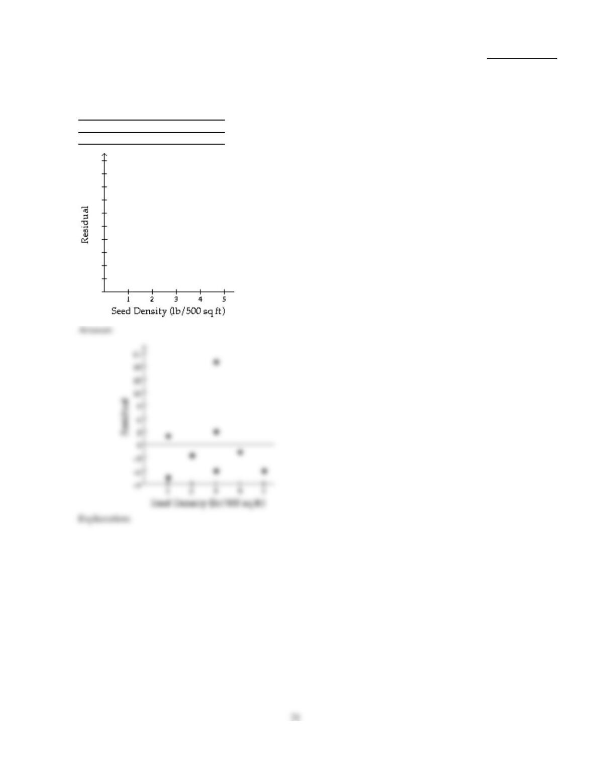
A grass seed company conducts a study to determine the relationship between the density
of seeds planted (in pounds per 500 sq ft) and the quality of the resulting lawn. Eight
similar plots of land are selected and each is planted with a particular density of seed. One
month later the quality of each lawn is rated on a scale of 0 to 100. The sample data are
given below, where x denotes seed density, and y denotes lawn quality.
x 1 1 2 3 3 3 4 5
y 30 40 40 40 50 65 50 50 y= 33.14 + 4.54x
47)
48)
^
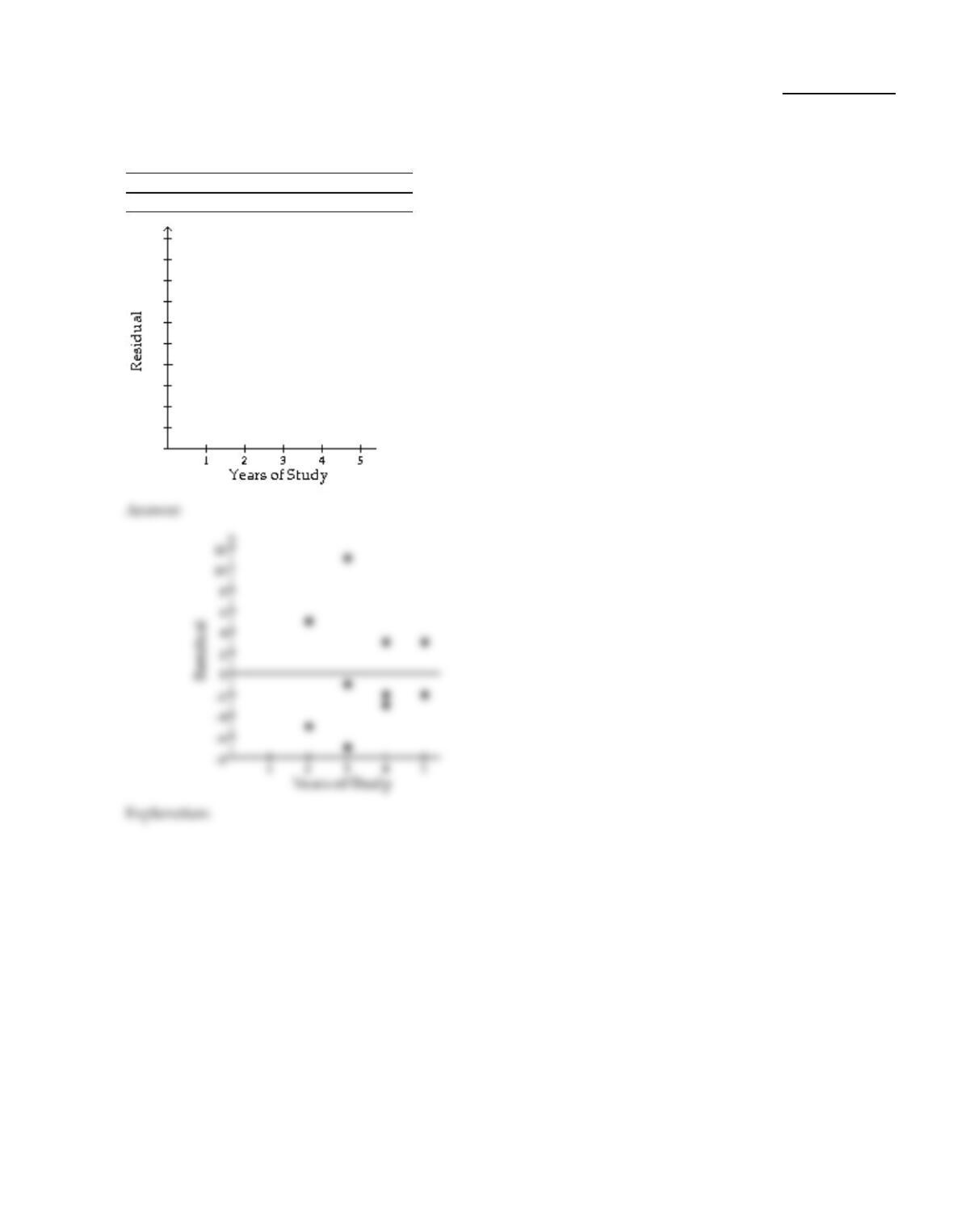
Applicants for a particular job, which involves extensive travel in Spanish speaking
countries, must take a proficiency test in Spanish. The sample data below were obtained in
a study of the relationship between the numbers of years applicants have studied Spanish
(x) and their score on the test (y).
x 3 4 4 2 5 3 4 5 3 2
y 57 78 72 58 89 63 73 84 75 48 y= 31.55 + 10.90x
48)
22
49)
^
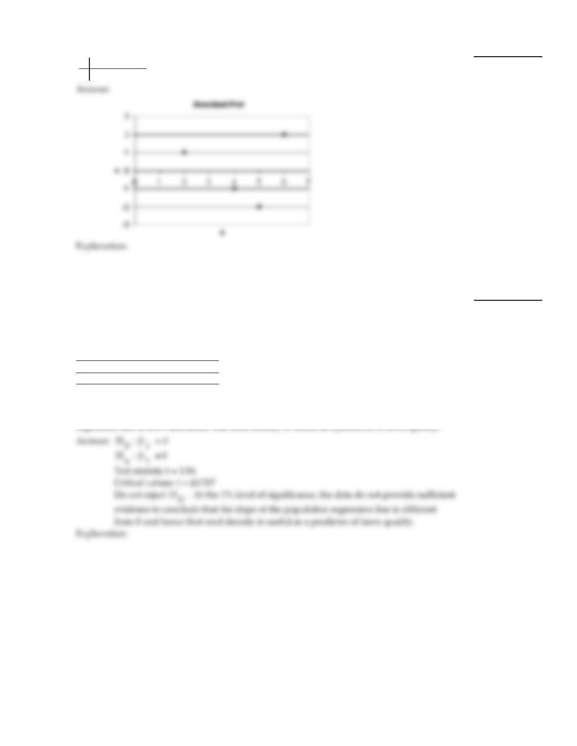
x 2 4 5 6
y 7 11 13 20 y= 3x
49)
Decide, at the given significance level, whether the data provide sufficient evidence to conclude that x is useful for
predicting y.
50)
^
A grass seed company conducts a study to determine the relationship between the density
of seeds planted (in pounds per 500 sq ft) and the quality of the resulting lawn. Eight
similar plots of land are selected and each is planted with a particular density of seed. One
month later the quality of each lawn is rated on a scale of 0 to 100. The sample data are
given below, where x denotes seed density, and y denotes lawn quality.
x 1 1 2 3 3 3 4 5
y 30 40 40 40 50 65 50 50 y= 33.14 + 4.54x
The standard error of the estimate is approximately 9.074. At the 1% level of significance,
do the data provide sufficient evidence to conclude that the slope of the population
50)
23
Perform the required correlation test. You may presume that the assumptions for regression inferences are met.
51)
Ten students in a graduate program were randomly selected. Their grade point averages
(GPAs) when they entered the program were between 3.5 and 4.0. The following data
consist of the students’ GPAs (x) on entering the program and their current GPAs (y).
x 3.5 3.8 3.6 3.6 3.5 3.9 4.0 3.9 3.5 3.7
y 3.6 3.7 3.9 3.6 3.9 3.8 3.7 3.9 3.8 4.0
The sample linear correlation coefficient is r = 0.043. At the 5% significance level, do the
data provide sufficient evidence to conclude that entering GPA and current GPA are
linearly correlated?
51)
Provide an appropriate response.
52)
A researcher is interested in the relationship between age and income. He performs a
regression analysis using age as the predictor variable and annual income as the response
variable. He obtains the equation of the regression line and then computes the standard
error of the estimate, which comes out to $6570. Give an interpretation of the standard
error of the estimate.
52)
53)
In the context of regression analysis, explain what is meant by the term “residual”.
53)
54)
In the context of linear correlation, explain the difference between r and .
54)
24
55)
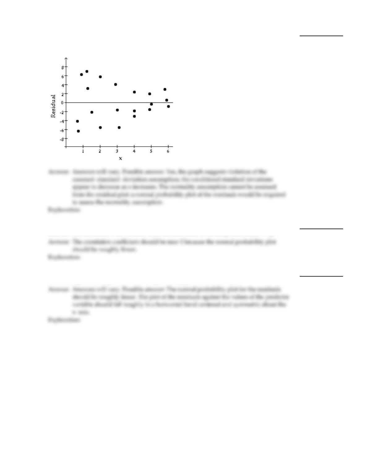
The graph below is a residual plot for a set of regression data. Does the graph suggest
violation of one or more of the assumptions for regression inferences? Explain your
answer.
55)
56)
What would you expect for the linear correlation coefficient between a set of sample data
and their normal scores if the variable under consideration is normally distributed. Why?
56)
57)
If the assumptions for regression inferences are met, what would you expect to see when
constructing a residual plot and a normal probability plot for the residuals?
57)
25
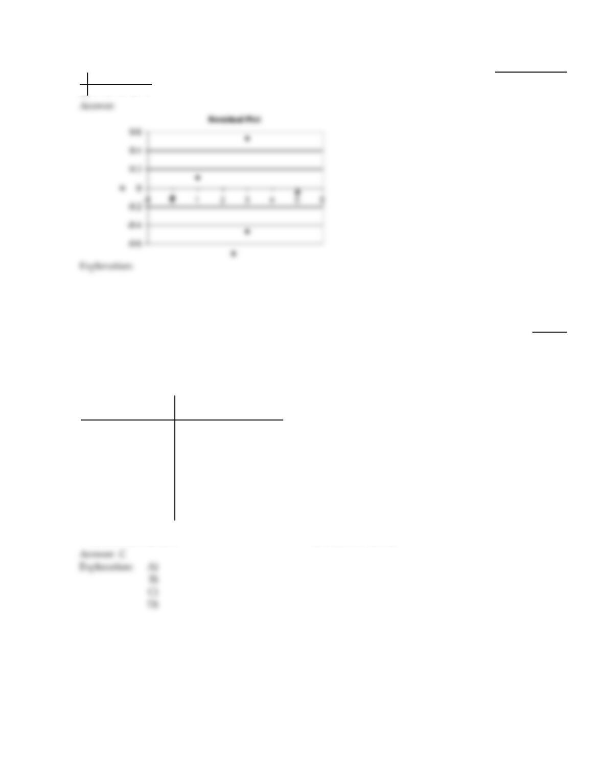
Construct a residual plot for the given data.
58)
^
x 0 1 5 3 3
y 7 5 –4 0 1 y= 7.105 – 2.211x
58)
MULTIPLE CHOICE. Choose the one alternative that best completes the statement or answers the question.
Provide an appropriate response.
59)
The maintenance costs incurred over the past year for a particular make, model, and year of
automobile are given below, along with each car’s end–of–year mileage. Assuming that there is a
relationship between milage and maintenance cost, use Minitab to find a 95% confidence interval
for the mean maintenance cost for all cars with this particular make, and model, that have been
driven 40,000 miles.
End–of–year mileage
(thousands of miles)
Last year’s maintenance
cost (dollars)
23.1
58.2
44.6
50.2
27.5
38.9
38.1
36.8
119
198
161
170
122
151
148
133
59)
A)
$146.88 to $155.09
B)
$135.49 to $166.47
C)
$145.82 to $156.15
D)
$138.68 to $163.29
26
60)
The table below gives the career free–throw percentage and the player height for a sample of NBA
basketball players, both past and present. Assuming that there is a relationship between height and
free–throw percentage, use Minitab to find a 95% confidence interval for the mean free–throw
percentage of all NBA players, past and present, with a playing height of 2.00 meters.
Height (meters) Career Free–throw %
1.83
2.16
2.13
2.26
2.11
2.01
1.83
1.98
76.0
54.2
71.0
81.1
75.6
78.2
90.4
82.1
Height (meters) Career Free–throw %
2.18
2.08
2.01
1.60
2.06
2.03
2.21
2.29
72.1
69.2
58.4
82.7
88.6
84.8
64.9
56.1
60)
A)
69.75% to 81.35%
B)
70.02% to 81.22%
C)
75.50% to 77.10%
D)
53.33% to 97.90%
61)
In a study of the relationship between weight and height, a sample regression equation is obtained,
in which height is used as the predictor variable. This sample regression equation is then used to
make inferences. Is it true or false that the point estimate of the mean weight of all subjects of
height 65 inches will be equal to the predicted weight of an individual of height 65 inches.?
61)
A)
True
B)
False
Obtain the required point estimate of the mean or predicted y–value. You may presume that the assumptions for
regression inferences are met and that x is useful as a predictor of y.
62)
^
Applicants for a particular job, which involves extensive travel in Spanish speaking countries,
must take a proficiency test in Spanish. The sample data below were obtained in a study of the
relationship between the numbers of years applicants have studied Spanish (x) and their score on
the test (y).
x 3 4 4 2 5 3 4 5 3 2
y 57 78 72 58 89 63 73 84 75 48 y= 31.55 + 10.90x
Use the data to predict the test score of an applicant who has studied Spanish for 2.1 years. Round
your answer to two decimal places.
62)
A)
52.55
B)
33.65
C)
42.45
D)
54.44
27
Provide an appropriate response.
63)
True or false? In the context of regression analysis, the sum of the residuals is always zero.
63)
A)
True
B)
False
Obtain the required prediction interval. You may presume that the assumptions for regression inferences are met.
64)
^
The sample data below are the index of exposure (x) to radioactive waste for nine different Oregon
counties and cancer mortality rate (y) (deaths per 100,000).
x 2.49 2.57 3.41 1.25 1.62 3.83 11.64 6.41 8.34
y 147.1 130.1 129.9 113.5 137.5 162.3 207.5 177.9 210.3 y= 114.72 + 9.23x
The standard error of the estimate is 14.0099. Determine a 95% prediction interval for the cancer
mortality rate of a county whose index of exposure is 3.87.
64)
A)
116.9 to 184.0 deaths per 100,000
B)
122.3 to 178.5 deaths per 100,000
C)
115.4 to 185.5 deaths per 100,000
D)
139.1 to 161.8 deaths per 100,000
65)
^
A grass seed company conducts a study to determine the relationship between the density of seeds
planted (in pounds per 500 sq ft) and the quality of the resulting lawn. Eight similar plots of land
are selected and each is planted with a particular density of seed. One month later the quality of
each lawn is rated on a scale of 0 to 100. The sample data are given below, where x denotes seed
density, and y denotes lawn quality.
x 1 1 2 3 3 3 4 5
y 30 40 40 40 50 65 50 50 y= 33.14 + 4.54x
The standard error of the estimate is se= 9.0736. Determine a 99% prediction interval for the lawn
quality of a lawn sown with a seed density of 1.4.
65)
A)
7.5 to 71.5
B)
3.9 to 75.1
C)
12.2 to 84.0
D)
22.3 to 56.6
Provide an appropriate response.
28
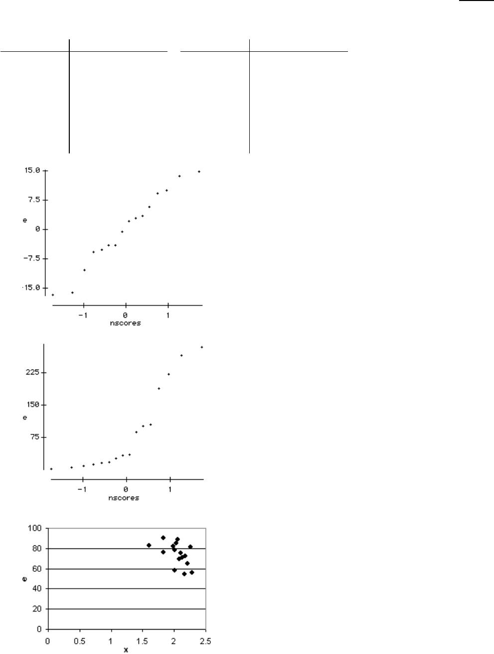
66)
The table below gives the career free–throw percentage and the player height for a sample of NBA
basketball players, both past and present. Assuming that the data can be modeled with a linear
model, use technology to obtain a normal probability plot of the residuals.
Height (meters) Career Free–throw %
1.83
2.16
2.13
2.26
2.11
2.01
1.83
1.98
76.0
54.2
71.0
81.1
75.6
78.2
90.4
82.1
Height (meters) Career Free–throw %
2.18
2.08
2.01
1.60
2.06
2.03
2.21
2.29
72.1
69.2
58.4
82.7
88.6
84.8
64.9
56.1
66)
A)
B)
C)
29
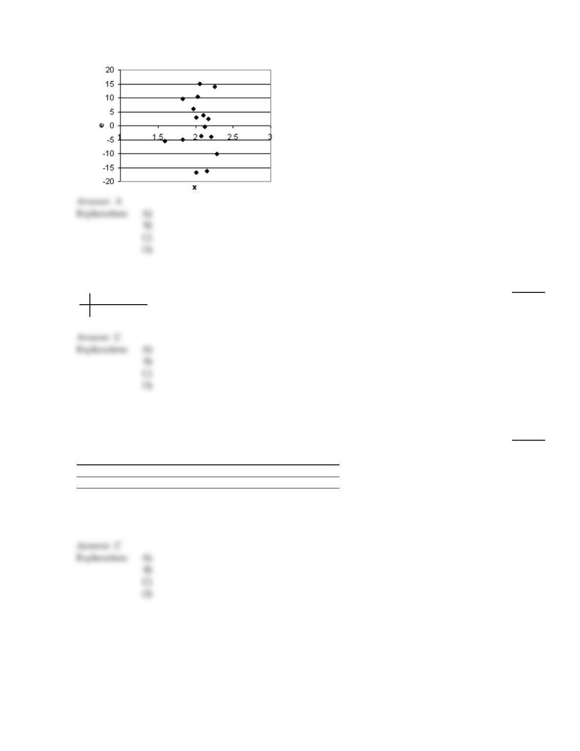
D)
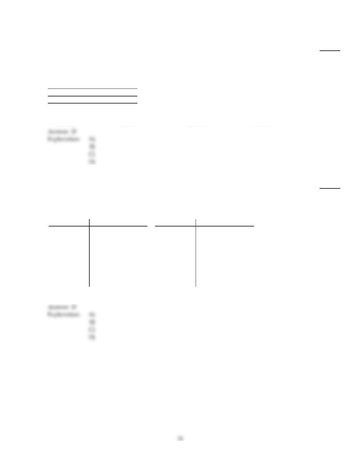
Determine the standard error of the estimate.
67)
^
x 2 4 5 6
y 7 11 13 20 y= 3x
67)
A)
6.2750
B)
4.1892
C)
2.2361
D)
5.00
Obtain the required confidence interval for the slope of the population regression line. You may presume that the
assumptions for regression inferences are met.
68)
^
The sample data below are the index of exposure (x) to radioactive waste for nine different Oregon
counties and cancer mortality rate (y) (deaths per 100,000).
x 2.49 2.57 3.41 1.25 1.62 3.83 11.64 6.41 8.34
y 147.1 130.1 129.9 113.5 137.5 162.3 207.5 177.9 210.3 y= 114.72 + 9.23x
The standard error of the estimate is approximately 14.0099. Find a 99% confidence interval for
the slope of the population regression line that relates cancer mortality rate to index of exposure.
68)
A)
5.11 to 13.35
B)
4.46 to 14.00
C)
4.26 to 14.20
D)
4.97 to 13.49
30
Obtain the required point estimate of the mean or predicted y–value. You may presume that the assumptions for
regression inferences are met and that x is useful as a predictor of y.
69)
^
A grass seed company conducts a study to determine the relationship between the density of seeds
planted (in pounds per 500 sq ft) and the quality of the resulting lawn. Eight similar plots of land
are selected and each is planted with a particular density of seed. One month later the quality of
each lawn is rated on a scale of 0 to 100. The sample data are given below, where x denotes seed
density, and y denotes lawn quality.
x 1 1 2 3 3 3 4 5
y 30 40 40 40 50 65 50 50 y= 33.14 + 4.54x
Round your answer to two decimal places.
69)
A)
42.08
B)
37.54
C)
55.14
D)
53.12
Provide an appropriate response.
70)
The table below gives the career free–throw percentage and the player height for a sample of NBA
basketball players, both past and present. Assuming that there is a relationship between height and
free–throw percentage, use Minitab to find a 95% prediction interval for the mean free–throw
percentage of Kevin Garnett, who is 2.00 meters tall.
Height (meters) Career Free–throw %
1.83
2.16
2.13
2.26
2.11
2.01
1.83
1.98
76.0
54.2
71.0
81.1
75.6
78.2
90.4
82.1
Height (meters) Career Free–throw %
2.18
2.08
2.01
1.60
2.06
2.03
2.21
2.29
72.1
69.2
58.4
82.7
88.6
84.8
64.9
56.1
70)
A)
75.50% to 77.10%
B)
70.00% to 81.20%
C)
69.75% to 81.35%
D)
53.33% to 97.90%
Determine the standard error of the estimate.
71)
Two different tests are designed to measure employee dexterity and productivity. Several
employees are randomly selected and tested with the results below. Here, x denotes dexterity
score, and y denotes productivity score.
x
y
23 25 28 21 21 25 26 30 34 36
49 53 59 42 47 53 55 63 67 75
71)
A)
3.8926
B)
1.753
C)
1.6511
D)
3.6700
Provide an appropriate response.
72)
The table below gives the career free–throw percentage and the player height for a sample of NBA
basketball players, both past and present. Use technology to compute a p–value and use it to
determine whether the regression equation is useful for making predictions about freethrow
percentage. Test at the 10% significance level with the hypotheses H0: 1= 0 and Ha: 1
0.
Height (meters) Career Free–throw %
1.83
2.16
2.13
2.26
2.11
2.01
1.83
1.98
76.0
54.2
71.0
81.1
75.6
78.2
90.4
82.1
Height (meters) Career Free–throw %
2.18
2.08
2.01
1.60
2.06
2.03
2.21
2.29
72.1
69.2
58.4
82.7
88.6
84.8
64.9
56.1
72)
A)
p = 0.04622. Since p <, do not reject the null hypothesis. The regression equation is not
useful for making free throw percentage predictions.
B)
p = 0.04622. Since p <, reject the null hypothesis. The regression equation is useful for
making free throw percentage predictions.
C)
p = 0.02311. Since p <, reject the null hypothesis. The regression equation is useful for
making free throw percentage predictions.
D)
p = 0.02311. Since p <, do not reject the null hypothesis. The regression equation is not
useful for making free throw percentage predictions.
Obtain the required confidence interval for the slope of the population regression line. You may presume that the
assumptions for regression inferences are met.
73)
^
Applicants for a particular job, which involves extensive travel in Spanish speaking countries,
must take a proficiency test in Spanish. The sample data below were obtained in a study of the
relationship between the numbers of years applicants have studied Spanish (x) and their score on
the test (y).
x 3 4 4 2 5 3 4 5 3 2
y 57 78 72 58 89 63 73 84 75 48 y= 31.55 + 10.90x
The standard error of the estimate is approximately 5.651. Find a 99% confidence interval for the
slope of the population regression line that relates test score to number of years of study.
73)
A)
5.05 to 16.75
B)
5.23 to 16.57
C)
9.09 to 12.7
D)
25.70 to 37.40
Determine the standard error of the estimate.
74)
^
x 3 2 5 8
y 4 110 19 y= – 5 + 3x
74)
A)
1.29
B)
0
C)
0.17
D)
2.06
D)
Obtain the required confidence interval for the conditional mean. You may presume that the assumptions for regression
inferences are met.
75)
^
Find a 95% confidence interval for the conditional mean of the response variable at x =3.
x 0 1 5 3 3
y 7 5 –4 0 1 y= 7.105 – 2.211x
75)
A)
0.006 to 0.938
B)
–0.63 to 0.63
C)
–0.158 to 1.102
D)
–0.078 to 1.022
D)
33
D)
Obtain the required point estimate of the mean or predicted y–value. You may presume that the assumptions for
regression inferences are met and that x is useful as a predictor of y.
76)
^
The sample data below are the index of exposure (x) to radioactive waste for nine different Oregon
counties and cancer mortality rate (y) (deaths per 100,000).
x 2.49 2.57 3.41 1.25 1.62 3.83 11.64 6.41 8.34
y 147.1 130.1 129.9 113.5 137.5 162.3 207.5 177.9 210.3 y= 114.72 + 9.23x
Use the data to obtain an estimate of the mean cancer mortality rate for all counties whose index of
exposure is 3.26. Round your answer to one decimal place.
76)
A)
143.7 deaths per 100,000
B)
144.8 deaths per 100,000
C)
127.2 deaths per 100,000
D)
146.3 deaths per 100,000
77)
^
Determine a point estimate for the conditional mean at x =2.
x 3 2 4
y 8 4 6 y= 3 + x
77)
A)
4
B)
2
C)
3
D)
5
Provide an appropriate response.
78)
True or false? In the regression model, if 1= 0, then for each value x of the predictor variable, the
conditional distribution of the response variable is a normal distribution with a mean which is
independent of x.
78)
A)
True
B)
False
34
79)
The following table gives the US domestic oil production rates (excluding Alaska) over the past few
years. Assuming that the data can be modeled with a linear model, use technology to obtain the
standard error of the estimate.
Year Millions of barrels per day
1987 6.39
1988 6.12
1989 5.74
1990 5.58
1991 5.62
1992 5.46
1993 5.26
1994 5.10
Year Millions of barrels per day
1995 5.08
1996 5.07
1997 5.16
1998 5.08
1999 4.83
2000 4.85
2001 4.84
2002 4.83
79)
A)
0.18065
B)
4.76095
C)
–0.9287
D)
0.86257
Obtain the required confidence interval for the slope of the population regression line. You may presume that the
assumptions for regression inferences are met.
80)
^
Find a 90% confidence interval for the slope of the population regression line.
x 3 2 4
y 8 4 6 y= 3 + x
80)
A)
–4.331 to 6.331
B)
–4.058 to 6.058
C)
–9.936 to 11.936
D)
–6.733 to 8.733
Provide an appropriate response.
81)
Suppose that variables x and y satisfy the assumptions for regression inferences. For samples of
size n, each with the same values for the predictor variable, what is the distribution of the slope b1,
of the sample regression line?
81)
A)
t–distribution with mean 1 and standard deviation / Sxx
B)
Normal with mean 1 and standard deviation se
C)
Normal with mean 1 and standard deviation / Sxx
D)
t–distribution with mean 1 and standard deviation se
35
Obtain the required prediction interval. You may presume that the assumptions for regression inferences are met.
82)
^
The sample data below are the typing speeds (in words per minute) and reading speeds (in words
per minute) of nine randomly selected secretaries. Here, x denotes typing speed, and y denotes
reading
speed.
x 60 56 52 63 70 58 44 79 62
y 370 551 528 348 645 454 503 618 500 y= 290.2 + 3.502x
The standard error of the estimate is se= 100.33479. Determine a 90% prediction interval for the
reading speed of a secretary whose typing speed is 61.
82)
A)
354.1 to 653.5 words per minute
B)
440.3 to 567.3 words per minute
C)
307.1 to 700.5 words per minute
D)
303.4 to 704.3 words per minute
83)
^
Applicants for a particular job, which involves extensive travel in Spanish speaking countries,
must take a proficiency test in Spanish. The sample data below were obtained in a study of the
relationship between the numbers of years applicants have studied Spanish (x) and their score on
the test (y).
x 3 4 4 2 5 3 4 5 3 2
y 57 78 72 58 89 63 73 84 75 48 y= 31.55 + 10.90x
The standard error of the estimate is se= 5.651. Determine a 95% prediction interval for the score of
an applicant who has studied Spanish for 2.6 years.
83)
A)
46.0 to 73.8
B)
54.4 to 65.4
C)
45.8 to 74.0
D)
48.5 to 71.3
36
Provide an appropriate response.
84)
The maintenance costs incurred over the past year for a particular make, model, and year of
automobile are given below, along with each car’s end–of–year mileage. Use technology to
compute a p–value and use it to determine whether the regression equation is useful for making
predictions about maintenance costs for this automobile model. Test at the 1% significance level
with the hypotheses H0: 1= 0 and Ha: 1
0. Make sure to eliminate any outliers and/or
influential points from the data.
End–of–year mileage
(thousands of miles)
Last year’s maintenance
cost (dollars)
23.1
58.2
44.6
50.2
27.5
38.9
38.1
36.8
119
198
161
270
122
151
148
133
84)
A)
p = 0.02317. Since p >, reject the null hypothesis. The regression equation is useful for
making maintenance cost predictions.
B)
p = 0.00014. Since p <, reject the null hypothesis. The regression equation is useful for
making maintenance cost predictions.
C)
p = 0.02317. Since p >, do not reject the null hypothesis. The regression equation is not
useful for making maintenance cost predictions.
D)
p = 0.00014. Since p <, do not reject the null hypothesis. The regression equation is not
useful for making maintenance cost predictions.
85)
True or false? When performing regression analysis, different samples will all yield the same
sample regression line.
85)
A)
True
B)
False
Determine the standard error of the estimate.
86)
^
x 3 2 4
y 8 4 6 y= 3 + x
86)
A)
2.00
B)
0.250
C)
1.1547
D)
2.4495
37
Obtain the required prediction interval. You may presume that the assumptions for regression inferences are met.
87)
^
Ten students in a graduate program were randomly selected. Their grade point averages (GPAs)
when they entered the program were between 3.5 and 4.0. The following data consist of the
students’ GPAs (x) on entering the program and their current GPAs (y).
x 3.5 3.8 3.6 3.6 3.5 3.9 4.0 3.9 3.5 3.7
y 3.6 3.7 3.9 3.6 3.9 3.8 3.7 3.9 3.8 4.0 y= 3.67 + 0.0313x
The standard error of the estimate is approximately 0.14521. Determine a 99% prediction interval
for the current GPA of a student with an entering GPA of 3.8.
87)
A)
3.30 to 4.28
B)
3.27 to 4.31
C)
3.61 to 3.97
D)
3.34 to 4.24
Obtain the required confidence interval for the slope of the population regression line. You may presume that the
assumptions for regression inferences are met.
88)
^
A grass seed company conducts a study to determine the relationship between the density of seeds
planted (in pounds per 500 sq ft) and the quality of the resulting lawn. Eight similar plots of land
are selected and each is planted with a particular density of seed. One month later the quality of
each lawn is rated on a scale of 0 to 100. The sample data are given below, where x denotes seed
density, and y denotes lawn quality.
x 1 1 2 3 3 3 4 5
y 30 40 40 40 50 65 50 50 y= 33.14 + 4.54x
The standard error of the estimate is approximately 9.0736. Find a 95% confidence interval for the
slope of the population regression line that relates lawn quality to seed density.
88)
A)
–1.30 to 10.38
B)
27.10 to 39.18
C)
–1.50 to 10.58
D)
–0.26 to 9.34
38
Obtain the required confidence interval for the conditional mean. You may presume that the assumptions for regression
inferences are met.
89)
^
The sample data below are the index of exposure (x) to radioactive waste for nine different Oregon
counties and cancer mortality rate (y) (deaths per 100,000).
x 2.49 2.57 3.41 1.25 1.62 3.83 11.64 6.41 8.34
y 147.1 130.1 129.9 113.5 137.5 162.3 207.5 177.9 210.3 y= 114.72 + 9.23x
The standard error of the estimate is 14.0099. Determine a 95% confidence interval for the mean
cancer mortality rate of all counties whose index of exposure is 4.45.
89)
A)
146.9 to 164.7 deaths per 100,000
B)
145.2 to 166.4 deaths per 100,000
C)
120.8 to 190.8 deaths per 100,000
D)
144.7 to 166.9 deaths per 100,000
Provide an appropriate response.
90)
The maintenance costs incurred over the past year for a particular make, model, and year of
automobile are given below, along with each car’s end–of–year mileage. Assuming that there is a
relationship between milage and maintenance cost, use Minitab to find a 95% prediction interval
for the mean maintenance cost of Joe’s car (that is this particular make and model) that has 40,000
miles on it.
End–of–year mileage
(thousands of miles)
Last year’s maintenance
cost (dollars)
23.1
58.2
44.6
50.2
27.5
38.9
38.1
36.8
119
198
161
170
122
151
148
133
90)
A)
$146.88 to $155.09
B)
$138.68 to $163.29
C)
$135.49 to $166.47
D)
$145.82 to $156.15
39
Obtain the required point estimate of the mean or predicted y–value. You may presume that the assumptions for
regression inferences are met and that x is useful as a predictor of y.
91)
^
The sample data below are the typing speeds (in words per minute) and reading speeds (in words
per minute) of nine randomly selected secretaries. Here, x denotes typing speed, and y denotes
reading
speed.
x 60 56 52 63 70 58 44 79 62
y 370 551 528 348 645 454 503 618 500 y= 290.2 + 3.502x
Use the data to predict the reading speed of a secretary whose typing speed is 65. Round your
answer to the nearest word.
91)
A)
531 words per minute
B)
499 words per minute
C)
355 words per minute
D)
518 words per minute
Obtain the required confidence interval for the slope of the population regression line. You may presume that the
assumptions for regression inferences are met.
92)
^
The sample data below are the typing speeds (in words per minute) and reading speeds (in words
per minute) of nine randomly selected secretaries. Here, x denotes typing speed, and y denotes
reading
speed.
x 60 56 52 63 70 58 44 79 62
y 370 551 528 348 645 454 503 618 500 y= 290.2 + 3.502x
The standard error of the estimate is approximately 100.33479. Find a 90% confidence interval for
the slope of the population regression line that relates reading speed to typing speed.
92)
A)
–1.42 to 8.42
B)
–3.05 to 10.05
C)
–1.48 to 8.48
D)
–3.17 to 10.17
40