Obtain the required confidence interval for the conditional mean. You may presume that the assumptions for regression
inferences are met.
93)
^
Applicants for a particular job, which involves extensive travel in Spanish speaking countries,
must take a proficiency test in Spanish. The sample data below were obtained in a study of the
relationship between the numbers of years applicants have studied Spanish (x) and their score on
the test (y).
x 3 4 4 2 5 3 4 5 3 2
y 57 78 72 58 89 63 73 84 75 48 y= 31.55 + 10.90x
The standard error of the estimate is se= 5.651. Determine a 95% confidence interval for the mean
score of all applicants who have studied Spanish for 4.2 years.
93)
A)
73.3 to 81.4
B)
63.4 to 91.3
C)
72.4 to 82.2
D)
72.3 to 82.3
Obtain the required point estimate of the mean or predicted y–value. You may presume that the assumptions for
regression inferences are met and that x is useful as a predictor of y.
94)
^
Applicants for a particular job, which involves extensive travel in Spanish speaking countries,
must take a proficiency test in Spanish. The sample data below were obtained in a study of the
relationship between the numbers of years applicants have studied Spanish (x) and their score on
the test (y).
x 3 4 4 2 5 3 4 5 3 2
y 57 78 72 58 89 63 73 84 75 48 y= 31.55 + 10.90x
Obtain an estimate of the mean score for all applicants who have studied Spanish for 2.1 years.
Round your answer to two decimal places.
94)
A)
52.55
B)
33.65
C)
42.45
D)
54.44
Provide an appropriate response.
95)
True or false? The sample linear correlation coefficient, r, measures the linear correlation of all
possible pairs of observations of the two variables.
95)
A)
True
B)
False
96)
The table below gives the career free–throw percentage and the player height for a sample of NBA
basketball players, both past and present. Assuming that the data can be modeled with a linear
model, use technology to obtain the standard error of the estimate.
Height (meters) Career Free–throw %
1.83
2.16
2.13
2.26
2.11
2.01
1.83
1.98
76.0
54.2
71.0
81.1
75.6
78.2
90.4
82.1
Height (meters) Career Free–throw %
2.18
2.08
2.01
1.60
2.06
2.03
2.21
2.29
72.1
69.2
58.4
82.7
88.6
84.8
64.9
56.1
96)
A)
10.0280
B)
9.3804
C)
2.7970
D)
2.9901
97)
True or false? In the context of regression, the term “confidence” is usually reserved for interval
estimates of parameters while the term “prediction” is used for interval estimates of variables.
97)
A)
True
B)
False
Determine the standard error of the estimate.
98)
^
x 0 1 5 3 3
y 7 5 –4 0 1 y= 7.105 – 2.211x
98)
A)
0.4189
B)
0.6483
C)
0.5130
D)
0.7280
Provide an appropriate response.
99)
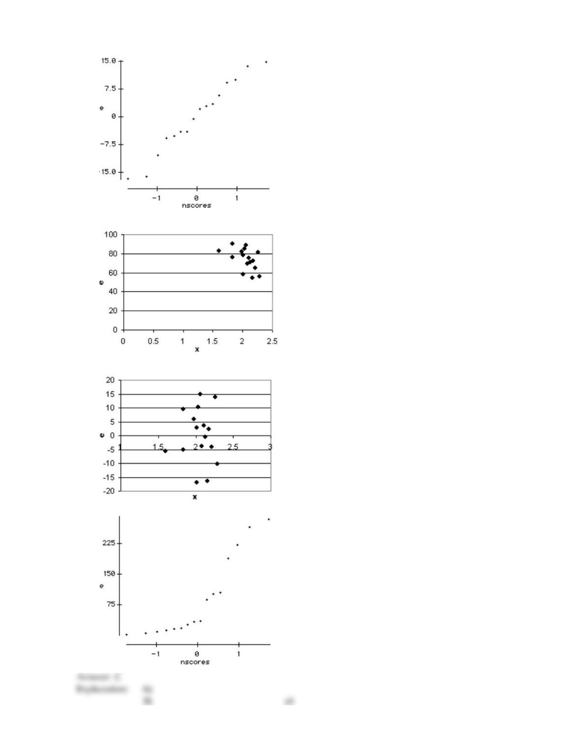
The table below gives the career free–throw percentage and the player height for a sample of NBA
basketball players, both past and present. Assuming that the data can be modeled with a linear
model, use technology to obtain a residual plot.
Height (meters) Career Free–throw %
1.83
2.16
2.13
2.26
2.11
2.01
1.83
1.98
76.0
54.2
71.0
81.1
75.6
78.2
90.4
82.1
Height (meters) Career Free–throw %
2.18
2.08
2.01
1.60
2.06
2.03
2.21
2.29
72.1
69.2
58.4
82.7
88.6
84.8
64.9
56.1
99)
42
A)
B)
C)
D)
Determine the standard error of the estimate.
100)
^
x 9 7 2 3 4 22 17
y 43 35 16 21 23 102 81 y= 6.18286 + 4.33937x
100)
A)
3.1270
B)
1.6419
C)
0.8275
D)
2.6959
Obtain the required confidence interval for the slope of the population regression line. You may presume that the
assumptions for regression inferences are met.
101)
^
A set of sample data consisting of 22 pairs of x and y values yields a regression equation of
y= 5.93 + 0.19x. The standard error of the estimate is approximately 12.40 and Sxx =95,830.
Obtain a 95% confidence interval for the slope of the population regression line that relates y to x.
101)
A)
0.11 to 0.27
B)
0.12 to 0.26
C)
0.09 to 0.29
D)
5.85 to 6.01
Obtain the required confidence interval for the conditional mean. You may presume that the assumptions for regression
inferences are met.
102)
^
The sample data below are the typing speeds (in words per minute) and reading speeds (in words
per minute) of nine randomly selected secretaries. Here, x denotes typing speed, and y denotes
reading
speed.
x 60 56 52 63 70 58 44 79 62
y 370 551 528 348 645 454 503 618 500 y= 290.2 + 3.502x
The standard error of the estimate is se= 100.33479. Determine a 90% confidence interval for the
mean reading speed of all secretaries whose typing speed is 49.
102)
A)
387.7 to 535.9 words per minute
B)
364.4 to 559.2 words per minute
C)
247.3 to 676.3 words per minute
D)
362.6 to 561.0 words per minute
103)
^
Find a 95% confidence interval for the conditional mean of the response variable at x =3.
x 3 2 4
y 8 4 6 y= 3 + x
103)
A)
–0.085 to 12.085
B)
–11.969 to 23.969
C)
–2.929 to 14.929
D)
22.969 to 28.969
Obtain the required prediction interval. You may presume that the assumptions for regression inferences are met.
104)
^
Find a 95% prediction interval for the value of the response variable at x =1.
x 0 1 5 3 3
y 7 5 –4 0 1 y= 7.105 – 2.211x
104)
A)
3.357 to 6.431
B)
3.758 to 6.03
C)
3.463 to 6.537
D)
3.553 to 6.235
Obtain the required point estimate of the mean or predicted y–value. You may presume that the assumptions for
regression inferences are met and that x is useful as a predictor of y.
105)
^
The sample data below are the index of exposure (x) to radioactive waste for nine different Oregon
counties and cancer mortality rate (y) (deaths per 100,000).
x 2.49 2.57 3.41 1.25 1.62 3.83 11.64 6.41 8.34
y 147.1 130.1 129.9 113.5 137.5 162.3 207.5 177.9 210.3 y= 114.72 + 9.23x
Use the data to predict the cancer mortality rate for a county whose index of exposure is 3.27.
Round your answer to one decimal place.
105)
A)
127.2 deaths per 100,000
B)
144.9 deaths per 100,000
C)
146.4 deaths per 100,000
D)
143.8 deaths per 100,000
Obtain the required prediction interval. You may presume that the assumptions for regression inferences are met.
106)
^
Find a 95% prediction interval for the value of the response variable at x =6.
x 2 4 5 6
y 7 11 13 20 y= 3x
106)
A)
9 to 27
B)
5.829 to 30.171
C)
9.741 to 26.259
D)
7.829 to 32.171
Obtain the required confidence interval for the slope of the population regression line. You may presume that the
assumptions for regression inferences are met.
107)
^
Ten students in a graduate program were randomly selected. Their grade point averages (GPAs)
when they entered the program were between 3.5 and 4.0. The following data consist of the
students’ GPAs (x) on entering the program and their current GPAs (y).
x 3.5 3.8 3.6 3.6 3.5 3.9 4.0 3.9 3.5 3.7
y 3.6 3.7 3.9 3.6 3.9 3.8 3.7 3.9 3.8 4.0 y= 3.67 + 0.0313x
The standard error of the estimate is approximately 0.14521. Obtain a 95% confidence interval for
the slope of the population regression line that relates current GPA to entering GPA.
107)
A)
–0.56 to 0.62
B)
–0.44 to 0.50
C)
–0.45 to 0.51
D)
–0.55 to 0.61
108)
^
Find a 90% confidence interval for the slope of the population regression line.
x 2 4 5 6
y 7 11 13 20 y= 3x
108)
A)
0.426 to 2.426
B)
0.793 to 5.207
C)
–0.612 to 2.612
D)
0.779 to 2.779
Obtain the required confidence interval for the conditional mean. You may presume that the assumptions for regression
inferences are met.
109)
^
Ten students in a graduate program were randomly selected. Their grade point averages (GPAs)
when they entered the program were between 3.5 and 4.0. The following data consist of the
students’ GPAs (x) on entering the program and their current GPAs (y).
x 3.5 3.8 3.6 3.6 3.5 3.9 4.0 3.9 3.5 3.7
y 3.6 3.7 3.9 3.6 3.9 3.8 3.7 3.9 3.8 4.0 y= 3.67 + 0.0313x
The standard error of the estimate is approximately 0.14521. Determine a 99% confidence interval
for the mean current GPA of all students with an entering GPA of 3.8.
109)
A)
3.61 to 3.97
B)
3.62 to 3.96
C)
3.27 to 4.31
D)
3.64 to 3.94
110)
^
A grass seed company conducts a study to determine the relationship between the density of seeds
planted (in pounds per 500 sq ft) and the quality of the resulting lawn. Eight similar plots of land
are selected and each is planted with a particular density of seed. One month later the quality of
each lawn is rated on a scale of 0 to 100. The sample data are given below, where x denotes seed
density, and y denotes lawn quality.
x 1 1 2 3 3 3 4 5
y 30 40 40 40 50 65 50 50 y= 33.14 + 4.54x
The standard error of the estimate is se= 9.0376. Determine a 99% confidence interval for the mean
lawn quality of all lawns sown with a seed density of 4.4.
110)
A)
30.8 to 71.8
B)
28.7 to 75.1
C)
34.0 to 72.3
D)
31.9 to 70.3
Determine the standard error of the estimate.
111)
The paired data below consists of test scores and hours of preparation for 5 randomly selected
students. Here, x denotes hours of preparation, and y denotes test score.
x 5 2 9 6 10
y 64 48 72 73 80
111)
A)
7.1720
B)
5.3999
C)
4.1097
D)
13.060
Obtain the required point estimate of the mean or predicted y–value. You may presume that the assumptions for
regression inferences are met and that x is useful as a predictor of y.
112)
^
The sample data below are the typing speeds (in words per minute) and reading speeds (in words
per minute) of nine randomly selected secretaries. Here, x denotes typing speed, and y denotes
reading
speed.
x 60 56 52 63 70 58 44 79 62
y 370 551 528 348 645 454 503 618 500 y= 290.2 + 3.502x
Use the data to obtain an estimate of the mean reading speed for all secretaries whose typing speed
is 67. Round your answer to the nearest word.
112)
A)
357 words per minute
B)
505 words per minute
C)
525 words per minute
D)
538 words per minute
113)
^
Determine the predicted value of the response variable at x =8.
x 3 2 5 8
y 4 110 19 y= – 5 + 3x
113)
A)
19
B)
8
C)
–37
D)
29
Provide an appropriate response.
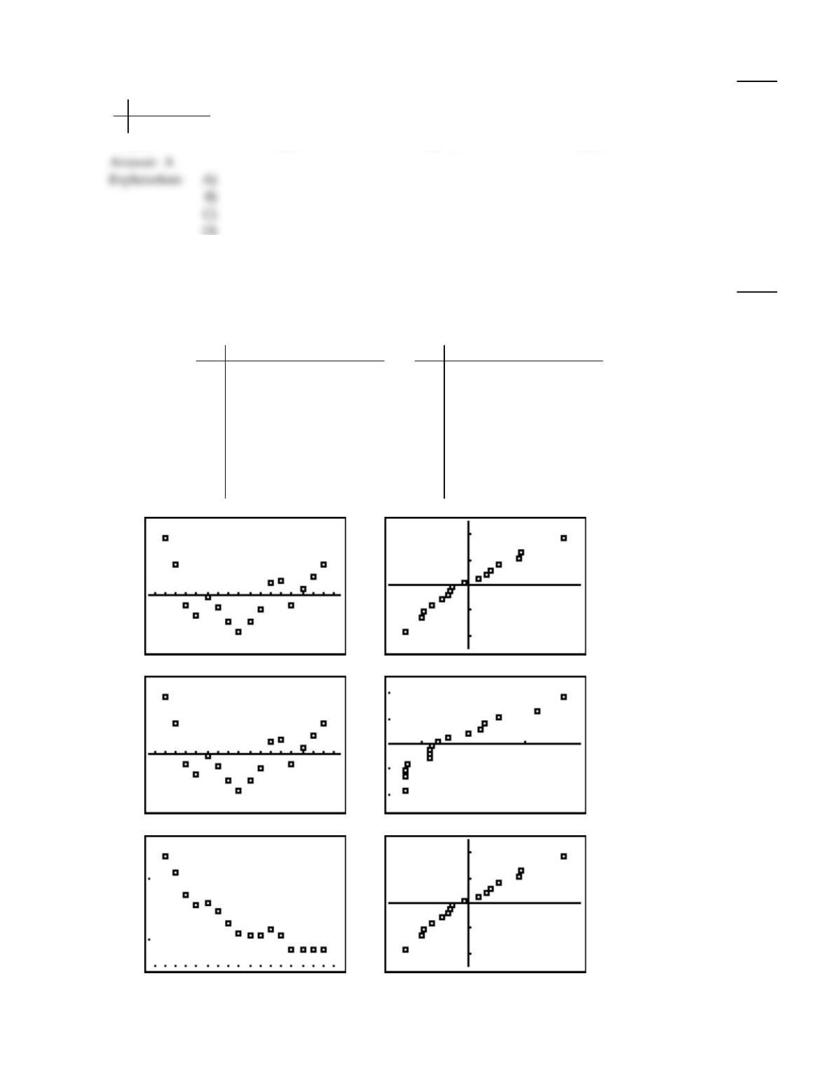
114)
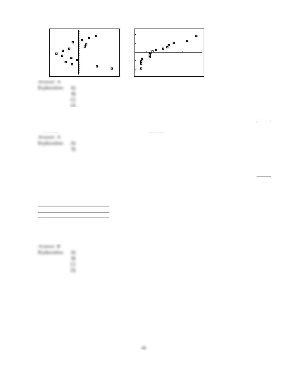
The following table gives the US domestic oil production rates (excluding Alaska) over the past few
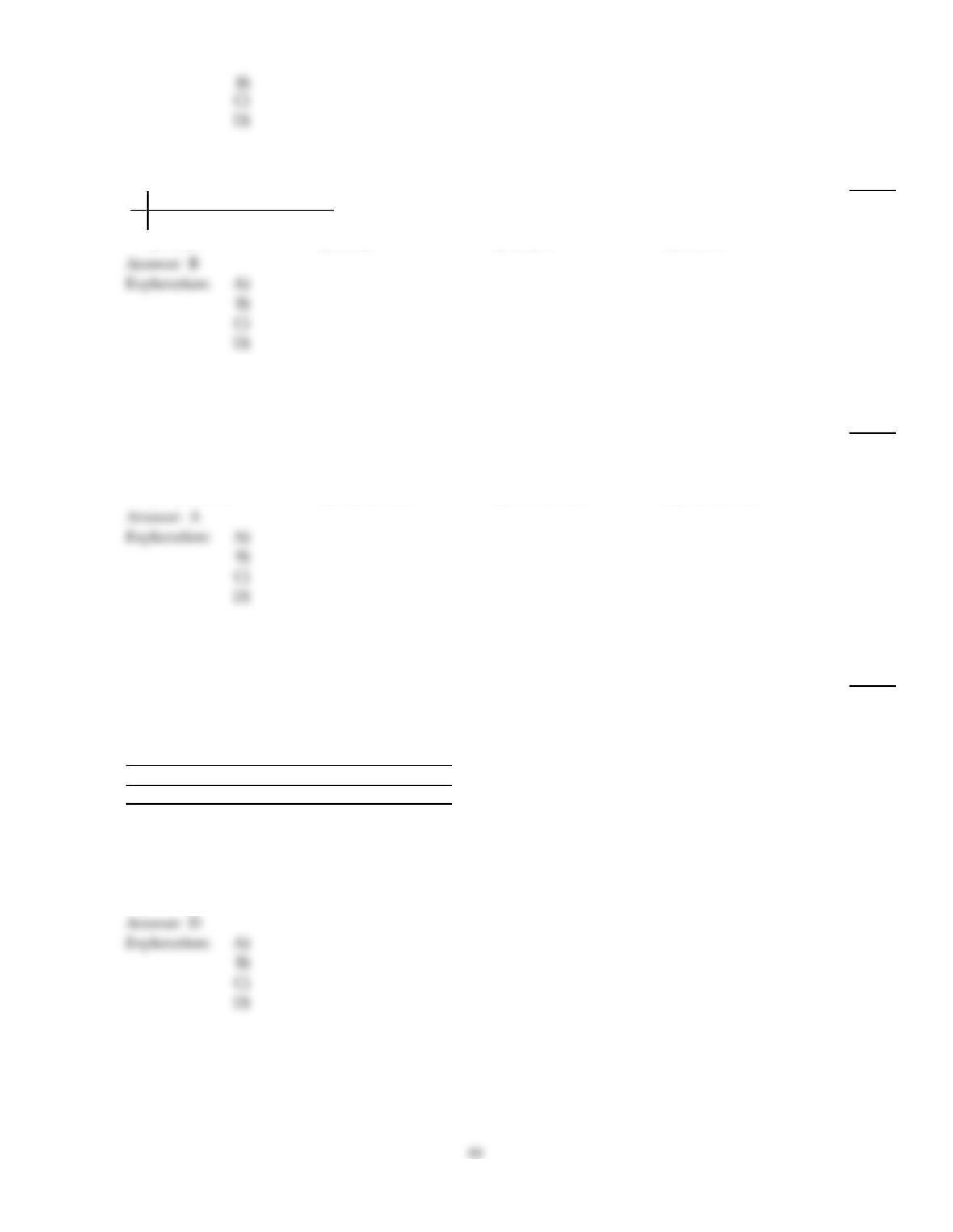
years. Assuming that the data can be modeled with a linear model, use technology to obtain a
residual plot and a normal probability plot of the residuals.
Year Millions of barrels per day
1987 6.39
1988 6.12
1989 5.74
1990 5.58
1991 5.62
1992 5.46
1993 5.26
1994 5.10
Year Millions of barrels per day
1995 5.08
1996 5.07
1997 5.16
1998 5.08
1999 4.83
2000 4.85
2001 4.84
2002 4.83
114)
A)
Residuals: Normal Probability Plot:
B)
Residuals: Normal Probability Plot:
C)
Residuals: Normal Probability Plot:
48
D)
Residuals: Normal Probability Plot:
115)
Is it true or false that the linear correlation coefficient between a set of sample data and their normal
scores cannot be negative?
115)
A)
True
B)
False
Obtain the required point estimate of the mean or predicted y–value. You may presume that the assumptions for
regression inferences are met and that x is useful as a predictor of y.
116)
^
A grass seed company conducts a study to determine the relationship between the density of seeds
planted (in pounds per 500 sq ft) and the quality of the resulting lawn. Eight similar plots of land
are selected and each is planted with a particular density of seed. One month later the quality of
each lawn is rated on a scale of 0 to 100. The sample data are given below, where x denotes seed
density, and y denotes lawn quality.
x 1 1 2 3 3 3 4 5
y 30 40 40 40 50 65 50 50 y= 33.14 + 4.54x
Use the data to obtain an estimate of the mean lawn quality for all lawns sown with a seed density
of 2.3. Round your answer to two decimal places.
116)
A)
44.64
B)
43.58
C)
35.44
D)
39.98
Provide an appropriate response.
117)
When performing a hypothesis test for the population linear correlation coefficient, , the test
statistic is t = r/ (1 –r2)/(n – 2). What is the distribution of this test statistic if the null hypothesis,
H0: = 0, is true?
117)
A)
t–distribution with df = n – 1
B)
normal distribution
C)
chi–square distribution with df = n – 2
D)
t–distribution with df = n – 2
118)
^
A grass seed company conducts a study to determine the relationship between the density of seeds
planted (in pounds per 500 sq ft) and the quality of the resulting lawn. Eight similar plots of land
are selected and each is planted with a particular density of seed. One month later the quality of
each lawn is rated on a scale of 0 to 100. The sample data are given below, where x denotes seed
density, and y denotes lawn quality.
x 1 1 2 3 3 3 4 5
y 30 40 40 40 50 65 50 50 y= 33.14 + 4.54x
A 95% confidence interval for the slope of the population regression line that relates lawn quality to
seed density is –1.50 to 10.58. Which of the following is a correct interpretation of this confidence
interval? There may be more than one correct interpretation.
A: We can be 95% confident that the slope, 1, of the population regression line is between –1.50
and 10.58.
B: We can be 95% confident that with each unit increase in seed density, the increase in lawn
quality is somewhere between –1.50 and 10.58.
C: We can be 95% confident that with each unit increase in seed density, the increase in mean lawn
quality is somewhere between –1.50 and 10.58.
D: If seed density increases by one unit, there is a 95% chance that the increase in lawn quality lies
between –1.50 and 10.58.
118)
A)
A and B
B)
A, C, and D
C)
B and C
D)
A and C
D
Explanation:
Obtain the required confidence interval for the conditional mean. You may presume that the assumptions for regression
inferences are met.
119)
^
Find a 95% confidence interval for the conditional mean of the response variable at x =4.
x 2 4 5 6
y 7 11 13 20 y= 3x
119)
A)
7.121 to 16.879
B)
8.392 to 15.608
C)
6.121 to 15.879
D)
8.689 to 15.311
A
Explanation:
D
Explanation:
Provide an appropriate response.
120)
True or false? In the regression model, the predictor variable is useful in predicting the response
variable provided that 1= 0.
120)
A)
True
B)
False
121)
Wassamatta University offers supplemental instruction (SI) for introductory chemistry students
three times a week. The table below shows the number of SI visits during the semester for a sample
of students along with each student’s final class average. Use technology to compute a p–value and
use it to determine whether the regression equation is useful for making predictions about the
benefit of attending SI. Test at the 5% significance level with the hypotheses H0: 1= 0 and Ha: 1
0.
# of SI visits Final class average
2
8
10
9
15
7
5
4
81
85
76
76
72
72
42
59
# of SI visits Final class average
8
10
7
7
5
4
4
11
81
71
66
88
63
62
61
70
121)
A)
p = 0.0325. Since p <, do not reject the null hypothesis H0: 1= 0. The regression equation is
not useful for making predictions.
B)
p = 0.2529. Since p >, do not reject the null hypothesis H0: 1= 0. The regression equation is
not useful for making predictions.
C)
p = 0.04229. Since p <, reject the null hypothesis H0: 1= 0. The regression equation is
useful for making predictions.
D)
p = 0.2633. Since p >, reject the null hypothesis H0: 1= 0. The regression equation is useful
for making predictions.
Obtain the required confidence interval for the slope of the population regression line. You may presume that the
assumptions for regression inferences are met.
122)
^
Find a 90% confidence interval for the slope of the population regression line.
x 0 1 5 3 3
y 7 5 –4 0 1 y= 7.105 – 2.211x
122)
A)
2.387 to –2.035
B)
2.440 to –1.982
C)
–2.276 to –2.146
D)
(2.464 to –1.958