Find the value of the chi–square test statistic for the goodness–of–fit test.
107)
According to recent research, the distribution of the number of children per family in the U.S. is as
follows.
Number of children Percent
More than 3 20.3
321.3
214.5
116.1
027.8
A random sample of 700 families with both parents under 40 yielded the following data.
Number of children Number of families
More than 3 154
3196
246
1101
0203
You wish to test the claim that the distribution of the number of children per family for families
with both parents under 40 is the same as that of the U.S. as a whole. What is the value of the 2 test
statistic? Note that the expected frequencies are as follows: more than 3 children: 142.1;
3 children: 149.1; 2 children: 101.5; one child: 112.7; 0 children: 194.6.
107)
A)
2= 80.807
B)
2= 13.781
C)
2= 47.674
D)
2= 32.091
Find the specified conditional or marginal distribution for the given contingency table. Round to the nearest tenth of a
percent if needed.
108)
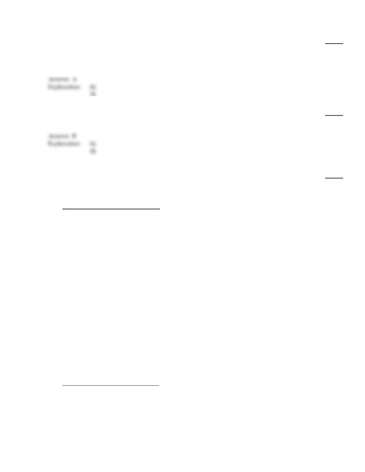
The contingency table below shows the income level for a random sample of adults cross classified
by sex.
26 24 29 79
29 30 28 87
55 54 57 166
Find the conditional distribution of the variable “income bracket” for men.
108)
A)
Low: 33.1% ; Middle: 32.5% ; High: 34.3%
B)
Male: 47.6% ; Female: 52.4%
C)
Low: 32.9% ; Middle: 30.4% ; High: 36.7%
D)
Low: 47.3% ; Middle: 44.4% ; High: 50.9%
Provide an appropriate response.
109)
Suppose that you wish to perform a chi–square test of independence. The two variables under
consideration are sex and blood type. True or false, if the two variables are not associated, we
would expect that the proportion of women in the sample with a given blood type would be
roughly equal to the proportion of men in the sample with the same blood type?
109)
A)
True
B)
False
110)
True or false, a 2–curve starts at 0 on the horizontal axis and extends indefinitely in both
directions approaching, but never touching, the horizontal axis as it does so?
110)
A)
True
B)
False
Group the bivariate data into a contingency table.
111)
The table below provides data on sex, political party affiliation, and income bracket for a sample of
people questioned during a poll. Group the bivariate data for the two variables “sex” and “income
bracket” into a contingency table.
Sex Political Party Income Bracket
M Rep High
F Dem Middle
F Dem Middle
M Dem Low
F Other Middle
M Rep Low
F Rep High
M Rep High
M Dem High
F Rep Low
M Dem High
F Rep Middle
F Dem Middle
M Dem Middle
M Rep Low
F Dem High
M Rep Low
F Other High
M Other Middle
F Dem Low
M Dem Middle
M Rep Low
F Dem Middle
111)
56
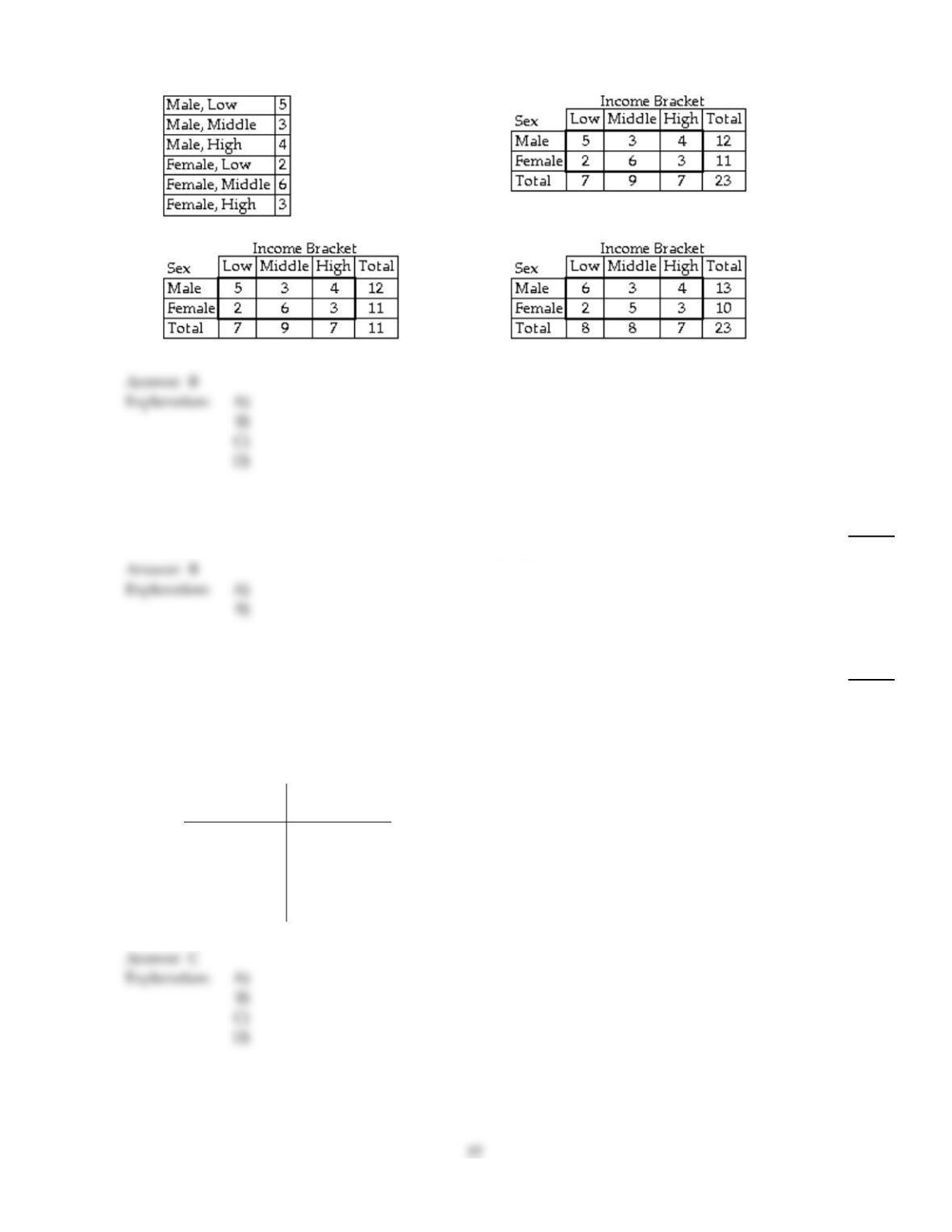
A)
B)
C)
D)
Provide an appropriate response.
112)
True or false, a 2–curve is symmetrical about 0?
112)
A)
True
B)
False
Find the value of the chi–square test statistic for the goodness–of–fit test.
113)
You wish to test the claim that workplace accidents are distributed on workdays as follows:
Monday: 25%, Tuesday: 15%, Wednesday: 15%, Thursday: 15%, Friday: 30%. In a study of 100
workplace accidents, 27 occurred on a Monday, 16 occurred on a Tuesday, 17 occurred on a
Wednesday, 14 occurred on a Thursday, and 26 occurred on a Friday. What is the value of the 2
test statistic? The observed frequencies and the expected frequencies are shown below.
Observed
Frequency (O)
Expected
Frequency (E)
27 25
16 15
17 15
14 15
26 30
113)
A)
2=3.714
B)
2=8.667
C)
2=1.093
D)
2=1.133
Find the required 2–value.
114)
For a 2–curve with 10 degrees of freedom, find the 2–value having area 0.99 to its right.
114)
A)
24.725
B)
4.865
C)
23.209
D)
2.558
Provide an appropriate response.
115)
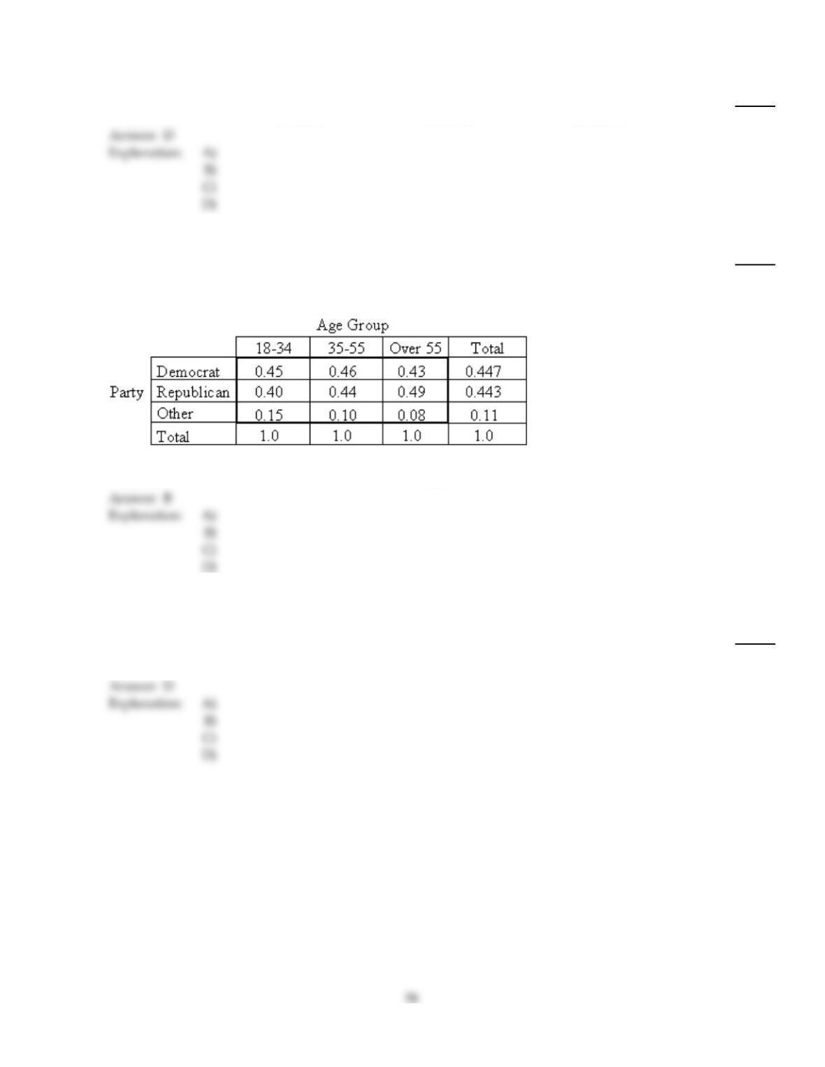
The table below shows the conditional distributions of the variable political party affiliation
corresponding to each age group for a certain population. What percentage of Democrats are aged
between 35 and 55? If it is not possible to tell from the table, say so.
115)
A)
34%
B)
It is not possible to tell from this table.
C)
46%
D)
44.7%
Find the required 2–value.
116)
For a 2–curve with 12 degrees of freedom, find 2
0.05 .
116)
A)
23.336
B)
19.675
C)
5.226
D)
21.026
Find the specified conditional or marginal distribution for the given contingency table. Round to the nearest tenth of a
percent if needed.
117)
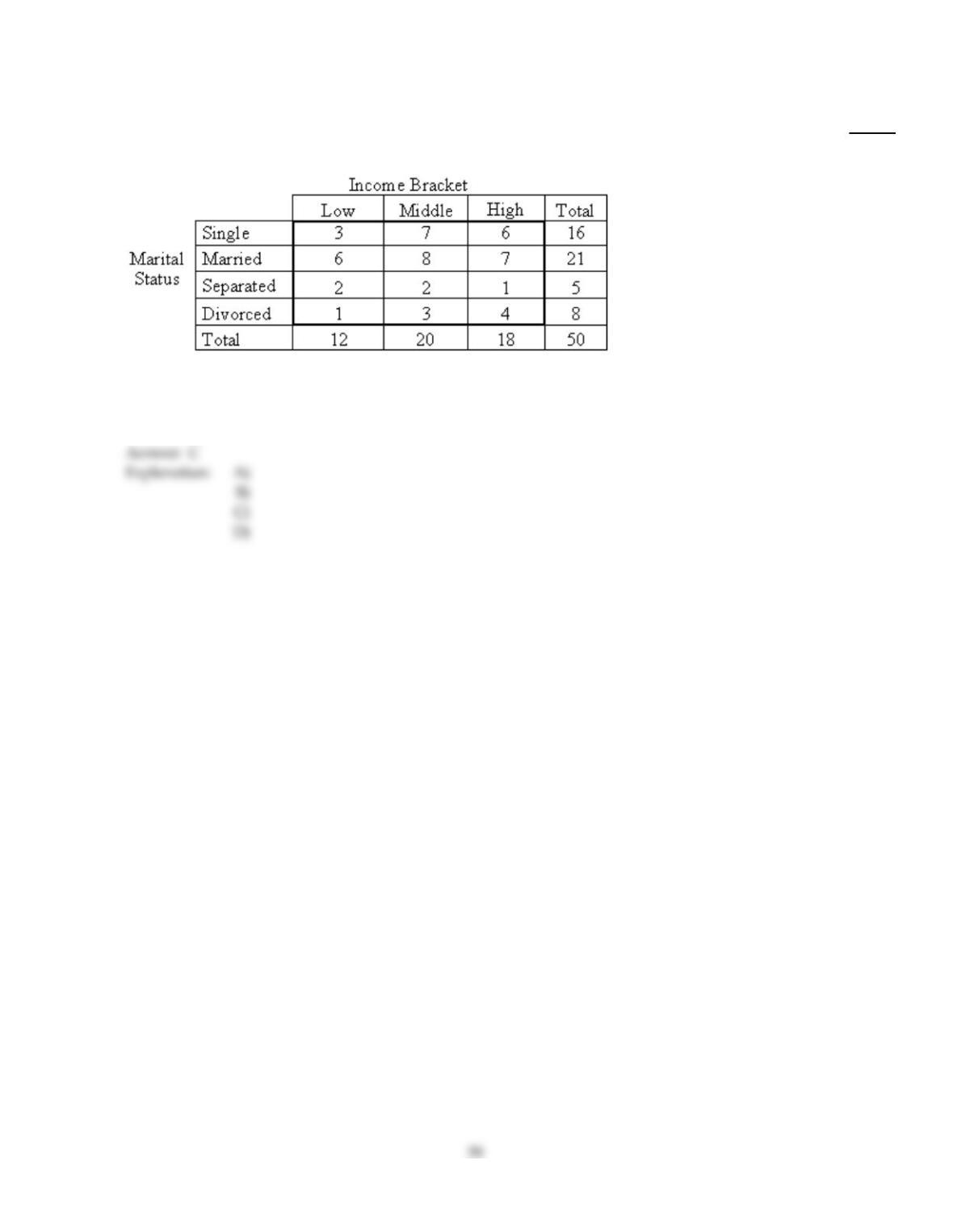
Use the given contingency table to find the marginal distribution of the
variable “income bracket”.
117)
A)
Low: 18.8%; Middle: 43.8%; High: 37.5%
B)
Low: 40%; Middle: 40%; High: 20%
C)
Low: 24%; Middle: 40%; High: 36%
D)
Single: 32%; Married: 42%; Separated: 10%; Divorced: 16%
Use the contingency table to solve the problem.
118)
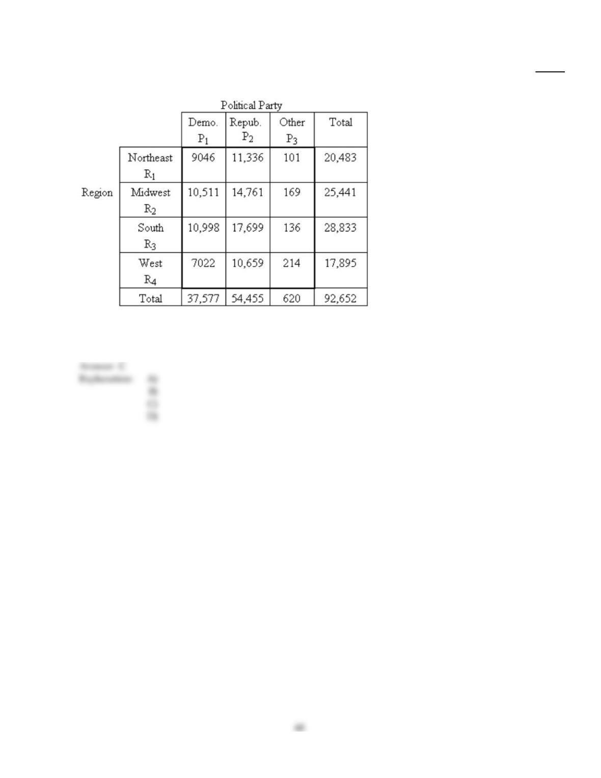
The following contingency table shows the popular votes cast in the 1984 presidential election cross
classified by region and political party. Data are in thousands, rounded to the nearest thousand.
What percentage of the voters were in the Midwest?
118)
A)
41.3%
B)
11.3%
C)
27.5%
D)
40.6%
Answer Key
Testname: C13
61
Answer Key
Testname: C13
62
Answer Key
Testname: C13
63
Answer Key
Testname: C13
64
Answer Key
Testname: C13
65
Answer Key
Testname: C13
66
Answer Key
Testname: C13
67
Answer Key
Testname: C13