Chapter 12 – Simulation
True / False
1. Simulation is an excellent technique to use when a situation is too complicated to use standard analytical procedures.
a.
True
b.
False
True
1
Introduction
2. Simulation is a trial-and-error approach to problem solving.
a.
True
b.
False
True
1
Introduction
3. The degree of risk is associated with the probability or magnitude of loss.
a.
True
b.
False
True
1
Simulation approach
4. To use Excel to generate a normally distributed random variable, you must know the mean and standard deviation of
the distribution and have a random number between 0 and 1.
a.
True
b.
False
True
1
Simulation approach
5. Trials of a simulation show what would happen when values of the probabilistic input change.
a.
True
b.
False
True
1
Simulation approach
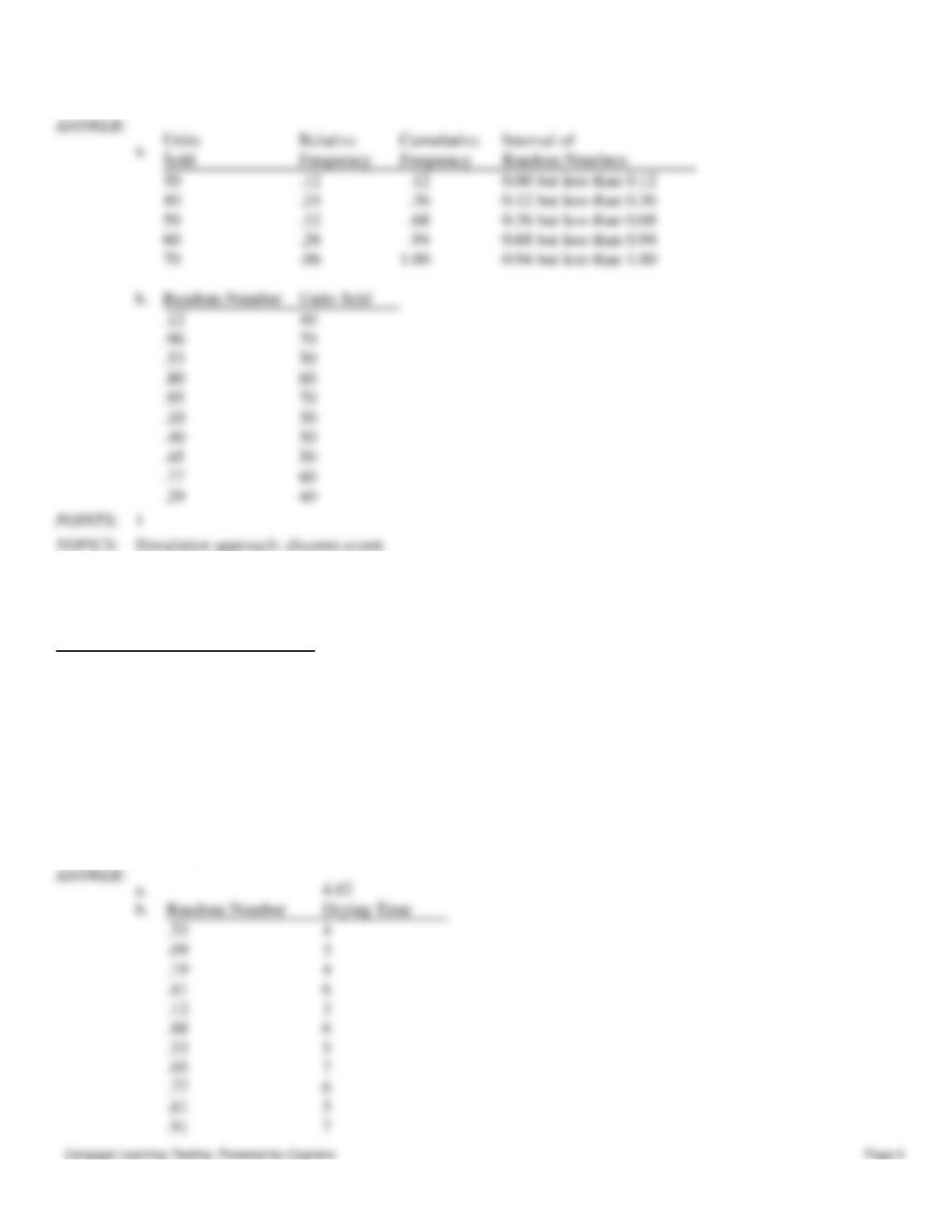
6. In a Monte Carlo simulation, each simulation trial is dependent upon the result of a previous trial.
a.
True
b.
False
False
1
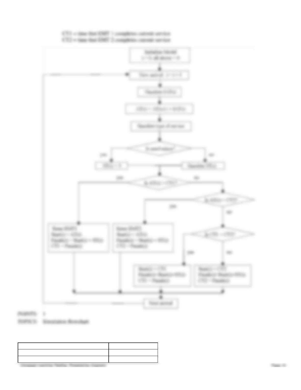
Monte Carlo simulation
7. Verification is the process of ensuring that the simulation model provides an accurate representation of the real system.
Chapter 12 – Simulation
a.
True
b.
False
False
1
8. In comparing different policies using simulation, one should use the same set of random numbers whenever possible.
a.
True
b.
False
True
1
9. Validation determines that the computer procedure is operating as it is intended to operate.
a.
True
b.
False
False
1
10. A discrete-event simulation reviews the status of the system periodically, whether or not an event occurs.
a.
True
b.
False
True
1
11. A static simulation model is used in situations where the state of the system affects how the system changes or evolves
over time.
a.
True
b.
False
False
1
12. For any waiting line system, (Average number of units in waiting line) = (Total waiting time) divided by (Total time
of simulation).
a.
True
b.
False
True
1
13. The parameters of a simulation model are the controllable inputs.
a.
True
Chapter 12 – Simulation
b.
False
False
1
14. Using simulation to perform risk analysis is like playing out many what-if scenarios by randomly generating values
for the probabilistic inputs.
a.
True
b.
False
True
1
15. Computer-generated random numbers are normally distributed over the interval from 0 to 1.
a.
True
b.
False
False
1
16. Computer-generated random numbers are not technically random.
a.
True
b.
False
True
1
17. Simulation is an optimization technique.
a.
True
b.
False
False
1
Introduction
18. Simulation models that must take into account how the system changes or evolves over time are referred to as
dynamic simulation models.
a.
True
b.
False
True
1
19. Computer-generated random numbers are normally distributed.
a.
True
b.
False
Chapter 12 – Simulation
False
1
Random numbers and generating probabilistic input values
20. Each simulation run provides only a sample of how the real system will operate.
a.
True
b.
False
True
1
Advantages and disadvantages of using simulation
21. One disadvantage of simulation is that it is limited in the variety of probability distributions that can be used in
modeling a system.
a.
True
b.
False
False
1
Simulation
22. A simulation model provides a convenient experimental laboratory for the real system.
a.
True
b.
False
True
1
Advantages and disadvantages of using simulation
23. Simulation allows the user to specify certain desired results (for example, profit or service level values), and then the
necessary model parameters and operating policies are determined.
a.
True
b.
False
False
1
Inventory simulation
Multiple Choice
24. A simulation model uses the mathematical expressions and logical relationships of the
a.
real system.
b.
computer model.
c.
performance measures.
d.
estimated inferences.
a
1
Introduction
25. Values for the probabilistic inputs to a simulation
Chapter 12 – Simulation
a.
are selected by the decision maker.
b.
are controlled by the decision maker.
c.
are randomly generated based on historical information.
d.
are calculated by fixed mathematical formulas.
c
1
Introduction
26. A quantity that is difficult to measure with certainty is called a
a.
risk analysis.
b.
project determinant.
c.
probabilistic input.
d.
profit/loss process.
c
1
Risk analysis
27. A value for probabilistic input from a discrete probability distribution
a.
is the value given by the RAND() function.
b.
is given by matching the probabilistic input with an interval of random numbers.
c.
is between 0 and 1.
d.
must be non-negative.
b
1
Simulation approach
28. The number of units expected to be sold is uniformly distributed between 300 and 500. If r is a random number
between 0 and 1, then the proper expression for sales is
a.
200(r)
b.
r + 300
c.
300 + 500(r)
d.
300 + r(200)
d
1
Simulation approach
29. When events occur at discrete points in time
a.
a simulation clock is required.
b.
the simulation advances to the next event.
c.
the model is a discrete-event simulation.
d.
All of the alternatives are correct.
d
1
Discrete-event simulation
30. If customer 2 has a service time of 1.6, and if customer 3 has an interarrival time of 1.1 and a service time of 2.3,
when will customer 3’s service be completed?
a.
5.0
b.
3.9
c.
3.4
d.
There is not enough information to answer.
d
1
Waiting line simulation
31. Common features of simulations—generating values from probability distributions, maintaining records, recording data
and summarizing results—led to the development of
a.
Excel and Lotus.
b.
BASIC, FORTRAN, PASCAL, and C.
c.
GPSS, SIMSCRIPT, SLAM, and Arena
d.
LINDO and The Management Scientist
c
1
Computer implementation
32. In order to verify a simulation model
a.
compare results from several simulation languages.
b.
be sure that the procedures for calculations are logically correct.
c.
confirm that the model accurately represents the real system.
d.
run the model long enough to overcome initial start-up results.
b
1
Verification and validation
33. Simulation
a.
does not guarantee optimality.
b.
is flexible and does not require the assumptions of theoretical models.
c.
allows testing of the system without affecting the real system.
d.
All of the alternatives are correct.
d
1
Advantages and disadvantages
34. A simulation model used in situations where the state of the system at one point in time does not affect the state of the
system at future points in time is called a
a.
dynamic simulation model.
b.
static simulation model.
c.
steady-state simulation model.
d.
discrete-event simulation model.
b
Chapter 12 – Simulation
35. The process of determining that the computer procedure that performs the simulation calculations is logically correct
is called
a.
implementation.
b.
validation.
c.
verification.
d.
repetition.
c
1
Other simulation issues
36. Numerical values that appear in the mathematical relationships of a model and are considered known and remain
constant over all trials of a simulation are
a.
parameters.
b.
probabilistic input.
c.
controllable input.
d.
events.
a
1
Other simulation issues
37. Which of the following statements is INCORRECT regarding the disadvantages of simulation?
a.
Each simulation run only provides a sample of how the real system will operate.
b.
The summary of the simulation data only provides estimates about the real system.
c.
The process of developing a simulation model of a complex system can be time-consuming.
d.
The larger the number of probabilistic inputs a system has, the less likely a simulation will provide the best
approach for studying the system.
d
1
Advantages and disadvantages of using simulation
38. Which of the following statements is INCORRECT regarding the advantages of simulation?
a.
Simulation is relatively easy to explain and understand.
b.
Simulation guarantees an optimal solution.
c.
Simulation models are flexible.
d.
A simulation model provides a convenient experimental laboratory for the real system.
b
1
Advantages and disadvantages of using simulation
39. The word “uniform” in the term “uniform random numbers” means
a.
all the numbers have the same number of digits.
b.
if one number is, say, 10 units above the mean, the next number will be 10 units below the mean.
1
Static simulation models
Chapter 12 – Simulation
c.
all the numbers are odd or all are even.
d.
each number has an equal probability of being drawn.
d
1
Random numbers and generating probabilistic input values
40. A table of uniformly distributed random numbers should be read
a.
from left to right.
b.
from top to bottom.
c.
diagonally, starting from the top left corner and moving to the bottom right.
d.
in any consistent sequence.
d
1
Random numbers and generating probabilistic input values
41. The process of generating probabilistic inputs and computing the value of the output is called
a.
simulation.
b.
verification.
c.
validation.
d.
implementation.
a
1
Simulation
42. A graphical tool that helps describe the logic of the simulation model is a
a.
Gantt chart.
b.
histogram.
c.
flowchart.
d.
stem-and-leaf display.
c
1
Subjective Short Answer
43. For the past 50 days, daily sales of laundry detergent in a large grocery store have been recorded (to the nearest 10).
Units Sold
Number of Times
30
8
40
12
50
15
60
10
70
5
a. Determine the relative frequency for each number of units sold.
b. Suppose that the following random numbers were obtained using Excel:
.12 .96 .53 .80 .95 .10 .40 .45 .77 .29
Use these random numbers to simulate 10 days of sales.
Chapter 12 – Simulation
.12
.36
.68
.94
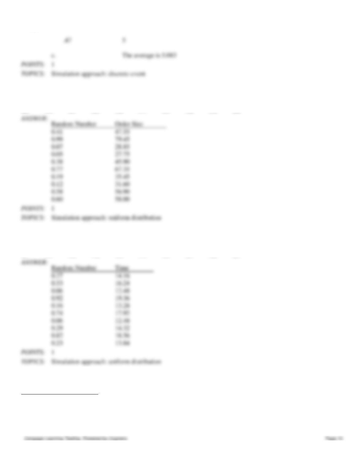
44. The drying rate in an industrial process is dependent on many factors and varies according to the following
distribution.
Minutes
Relative Frequency
3
.14
4
.30
5
.27
6
.18
7
.11
a. Compute the mean drying time.
b. Using these random numbers, simulate the drying time for 12 processes.
.33 .09 .19 .81 .12 .88 .53 .95 .77 .61 .91 .47
c. What is the average drying time for the 10 processes you simulated?
a.
Chapter 12 – Simulation
45. Greenfields is a mail order seed and plant business. The size of orders is uniformly distributed over the interval from
$25 to $80. Use the following random numbers to generate the size of 10 orders.
.41
.99
.07
.05
.38
.77
.19
.12
.58
.60
Random Number
Order Size
0.41
47.55
0.99
79.45
0.07
28.85
0.05
27.75
0.38
45.90
0.77
67.35
0.19
35.45
0.12
31.60
0.58
56.90
0.60
58.00
1
Simulation approach: uniform distribution
46. The time required to set up lighting for a portrait studio is uniformly distributed between 12 and 20 minutes. Use the
following random numbers to generate the setup time for 10 customers.
.27
.53
.06
.92
.16
.74
.06
.29
.82
.23
Random Number
Time
0.27
14.16
0.53
16.24
0.06
12.48
0.92
19.36
0.16
13.28
0.74
17.92
0.06
12.48
0.29
14.32
0.82
18.56
0.23
13.84
1
Simulation approach: uniform distribution
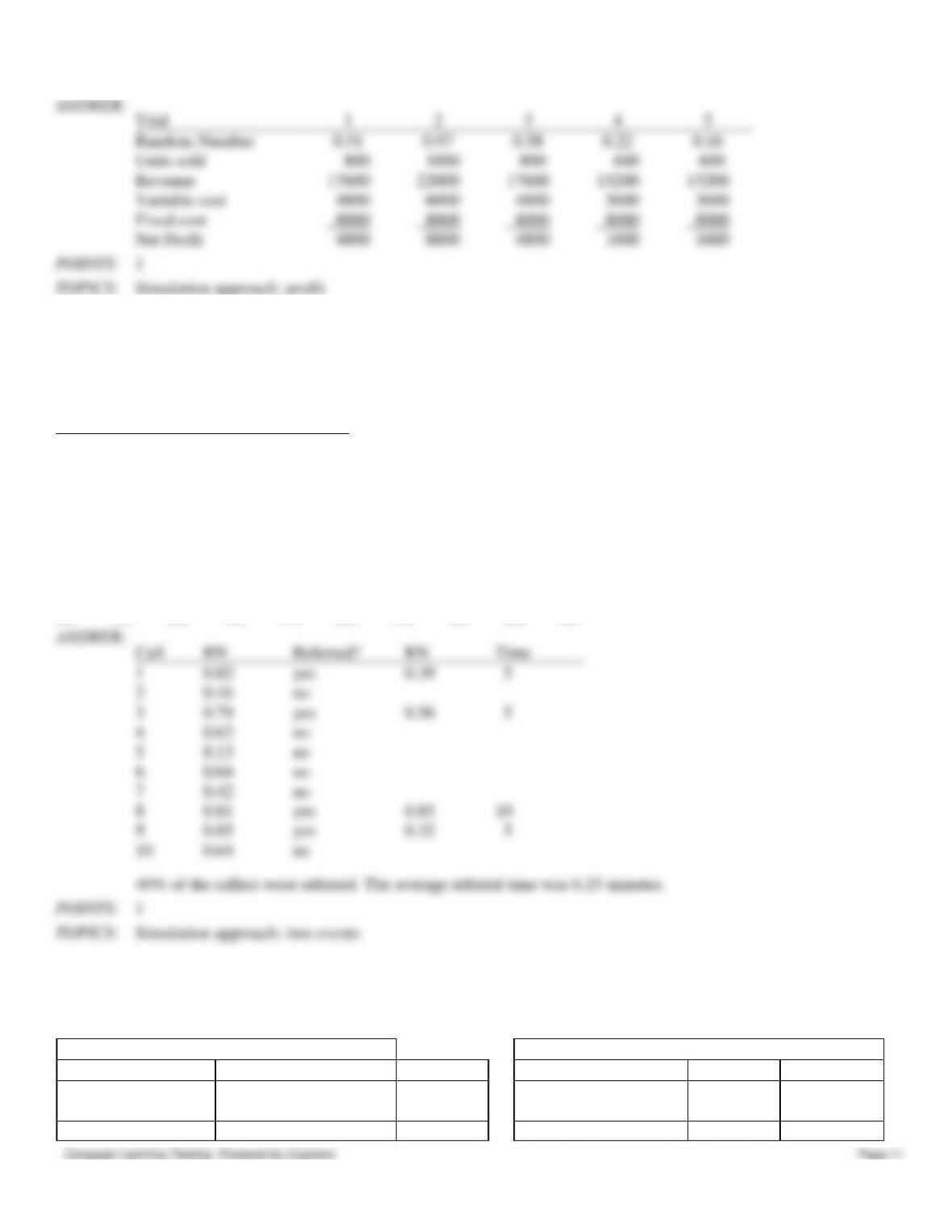
47. Estimates of the financial information for a new product show the following information:
Units Sold
Probability
Fixed cost
$8,000
600
.35
Variable cost
$6 / unit
800
.45
Revenue
$22 / unit
1000
.20
Use the random numbers .51, .97, .58, .22, and .16 to simulate five trials. What is the net profit for each trial?
.47
5
The average is 5.083
1
Simulation approach: discrete-event
Chapter 12 – Simulation
Trial
1
2
3
4
5
0.51
0.97
0.58
0.22
0.16
Revenue
48. Seventy-five percent of calls arriving at a help line can be handled by the person who answers the phone, but the
remaining 25% of them will need to be referred to someone else. Assume that every call requires one minute of attention
by the person who answers the phone (either to answer the question or to figure out how the referral should be handled).
Calls that are referred need an additional amount of time, as given in the table below.
Time Required
Probability
3 minutes
.25
5 minutes
.35
10 minutes
.40
Callers are served on a first come, first served basis, and are put on hold until the line is free. Use the random numbers to
simulate what happens to 10 callers. (Use the random numbers in order – from left to right, first row first – as you need
them.) What percentage of your callers needs to be referred? Of those who had to be referred, what is the average referral
time?
.82
.39
.16
.79
.56
.62
.13
.04
.42
.81
.85
.32
.64
.90
.73
.02
.76
.03
.86
.67
Call
Referred?
Time
0.82
yes
0.39
5
0.16
0.79
yes
0.56
5
0.62
0.13
0.04
0.42
0.81
yes
0.85
0.85
yes
0.32
5
0.64
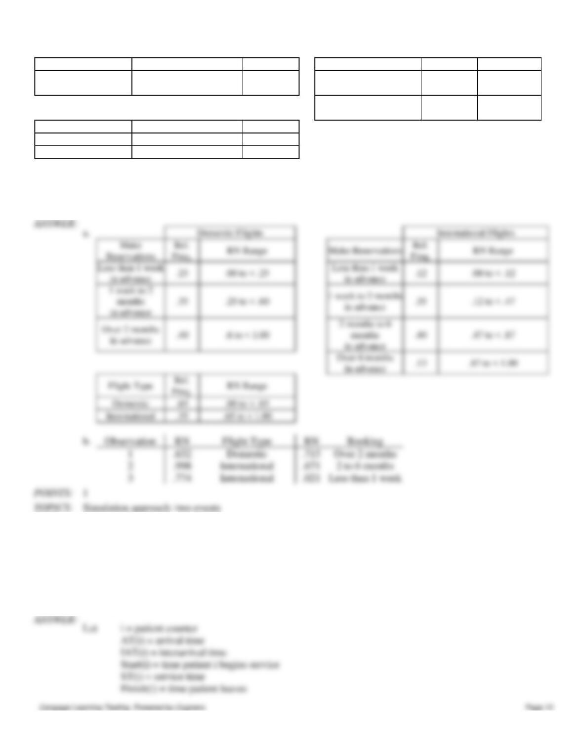
49. An airline reservation system first asks customers whether they want to schedule a domestic or an international flight.
Sixty-five percent of the reservations are for domestic flights. The time distribution of advance sales is also important, and
it is given below.
Domestic Flights
International Flights
Make Reservations
Rel. Freq.
RN Range
Make Reservations
Rel. Freq.
RN Range
Less than 1 week
in advance
.25
Less than 1 week
in advance
.12
1 week to 2 months
.35
1 week to 2 months
.35
Chapter 12 – Simulation
in advance
in advance
Over 2 months
in advance
.40
2 months to 6 months
in advance
.40
Over 6 months
In advance
.13
Flight Type
Rel. Freq.
RN Range
Domestic
.65
International
.35
a.
Place the appropriate random number ranges in the tables above.
b.
Set up and perform a simulation for three customers. Determine whether they want a
domestic or international flight, and how far in advance the reservation is being made. Use
random numbers from this list: .632 .715 .998 .671 .744 .021
a.
Flight Type
International
International
Simulation approach: two events
50. On a visit to an amusement park you pass someone who has just ridden a roller coaster and asks you for directions to
the First Aid Station. Realizing that traffic at the First Aid Station would be something to study with simulation, you
gather some information. Two EMTs staff the station, and patients wait and go to the first one available. People coming
there can be divided into two groups: those who need something minor (e.g. Tylenol, a band-aid) or those who need more
help. Assume those in the first group constitute 25% of the patients and take 5 minutes to have their problem solved.
Those in the second group need an uncertain amount of time, as given by a probability distribution. Develop a flowchart
for this simulation problem.
i = patient counter
AT(i) = arrival time
IAT(i) = interarrival time
Start(i) = time patient i begins service
ST(i) = service time
Finish(i) = time patient leaves
Chapter 12 – Simulation
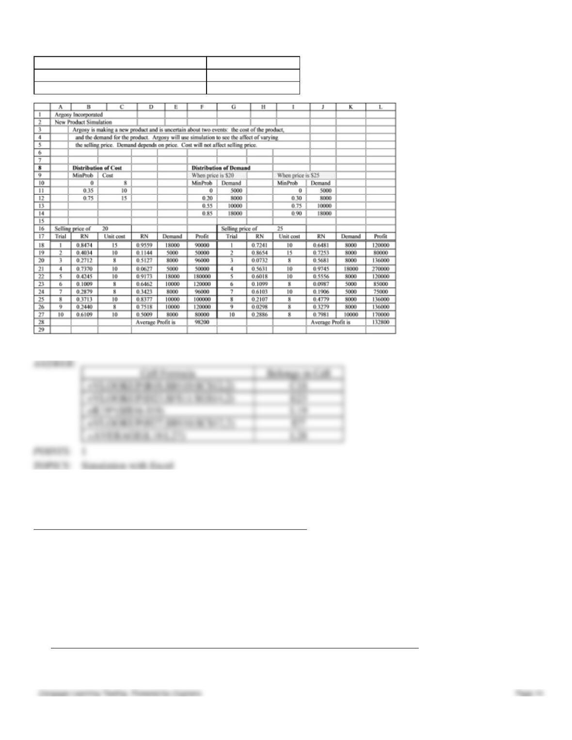
51. Using the spreadsheet below, give the cell address which would have the formula shown.
Cell Formula
Belongs in Cell
=VLOOKUP(B18,$B$10:$C$12,2)
=VLOOKUP(D23,$F$11:$G$14,2)
CT1 = time that EMT 1 completes current service
CT2 = time that EMT 2 completes current service
Simulation flowchart
Chapter 12 – Simulation
=K19*($I$16-I19)
=VLOOKUP(H27,$B$10:$C$12,2)
=AVERAGE(L18:L27)
=VLOOKUP(D23,$F$11:$G$14,2)
=K19*($I$16-I19)
=VLOOKUP(H27,$B$10:$C$12,2)
=AVERAGE(L18:L27)
1
Simulation with Excel
52. As the owner of a rent-a-car agency you have determined the following statistics:
Potential
Rentals Daily
Probability
Rental
Duration
Probability
0
.10
1 day
.50
1
.15
2 day
.30
2
.20
3 days
.15
3
.30
4 days
.05
4
.25
The gross profit is $40 per car per day rented. When there is demand for a car when none is available there is a goodwill
loss of $80 and the rental is lost. Each day a car is unused costs you $5 per car. Your firm initially has 4 cars.
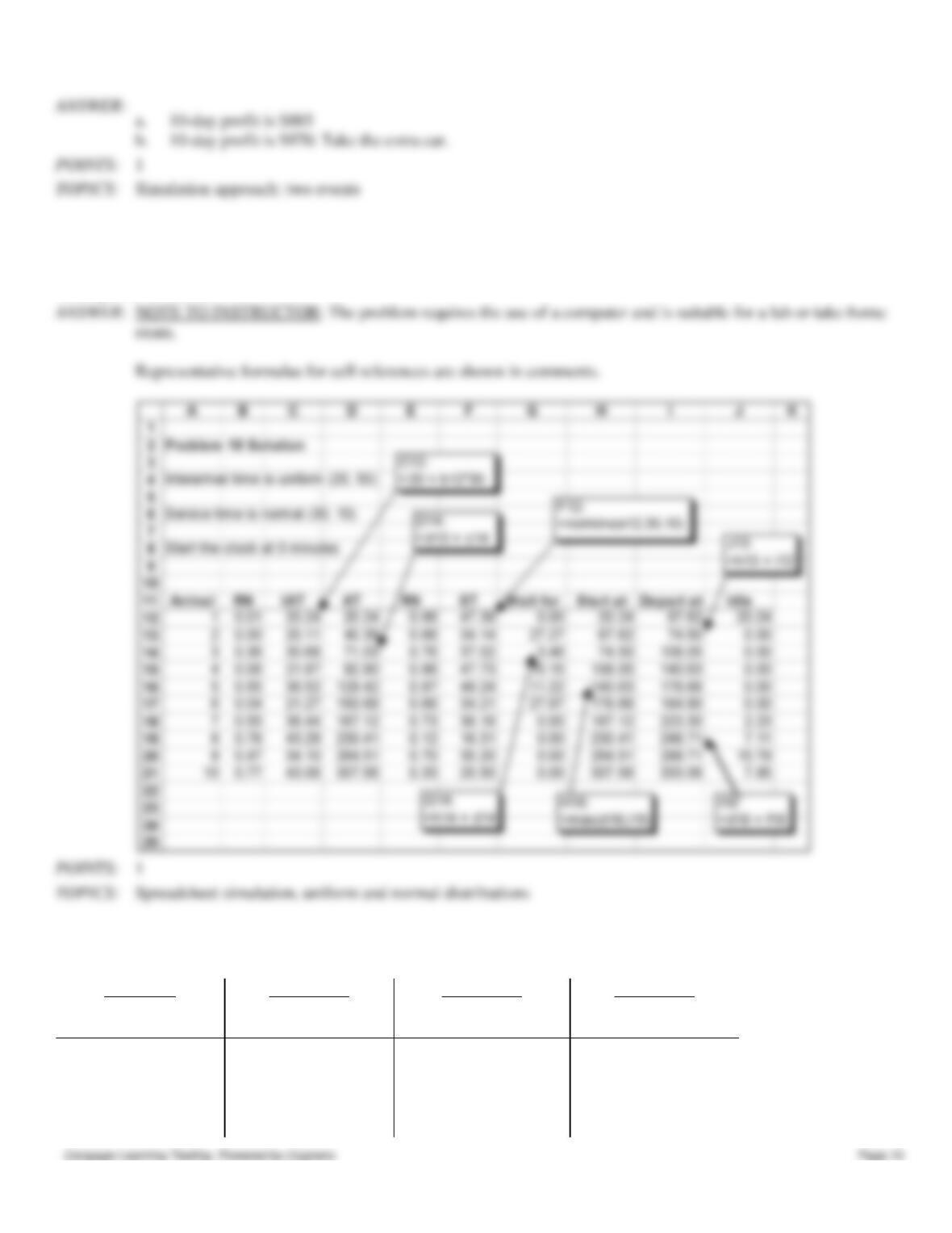
a. Conduct a 10-day simulation of this business using Row #1 below for demand and Row #2 below for rental length.
Row #1:
63
88
55
46
55
69
13
17
36
81
Row #2:
59
09
57
87
07
92
29
28
64
36
b. If your firm can obtain another car for $200 for 10 days, should you take the extra car?
Chapter 12 – Simulation
53. Arrivals to a truck repair facility have an interarrival time that is uniformly distributed between 20 and 50 minutes.
Service times are normally distributed with mean 30 minutes and standard deviation 10 minutes. Develop a spreadsheet
model to simulate the arrival of 100 trucks. Collect information on the time the repair facility is idle and on the average
waiting time for trucks.
54. Susan Winslow has two alternative routes to travel from her home in Olport to her office in Lewisburg. She can travel
on Freeway 5 to Freeway 57 or on Freeway 55 to Freeway 91. The time distributions are as follows:
Freeway 5
Freeway 57
Freeway 55
Freeway 91
Relative
Relative
Relative
Relative
Time
Frequency
Time
Frequency
Time
Frequency
Time
Frequency
5
.30
4
.10
6
.20
3
.30
6
.20
5
.20
7
.20
4
.35
7
.40
6
.35
8
.40
5
.20
8
.10
7
.20
9
.20
6
.15
8
.15
Chapter 12 – Simulation
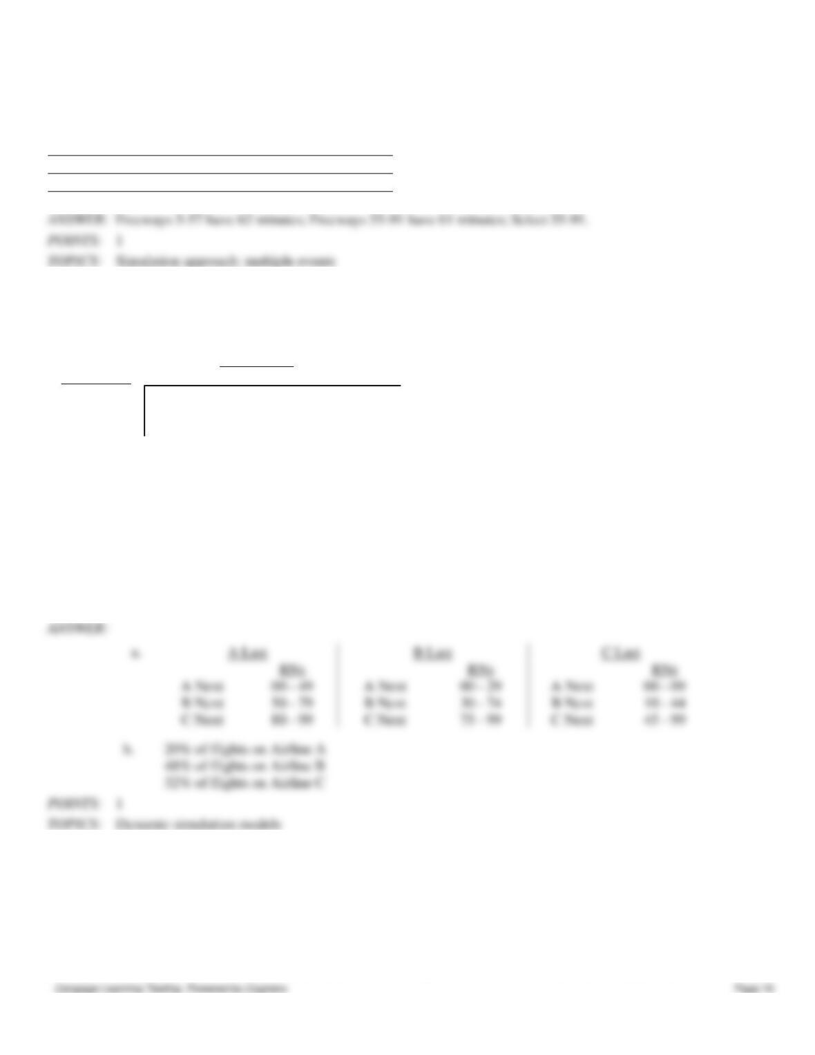
Do a five-day simulation of each of the two combinations of routes using the random numbers below. Based on this
simulation, which routes should Susan take if her objective is to minimize her total travel time?
Freeway 5
63
88
55
46
55
Freeway 57
59
09
57
87
07
Freeway 55
71
95
83
44
34
Freeway 91
51
79
09
67
15
Freeways 5-57 have 62 minutes; Freeways 55–91 have 61 minutes; Select 55–91.
1
Simulation approach: multiple events
55. Three airlines compete on the route between New York and Los Angeles. Stanton Marketing has performed an
analysis of first class business travelers to determine their airline choice. Stanton has modeled this choice as a Markov
process and has determined the following transition probabilities.
Next Airline
Last Airline
A
B
C
A
.50
.30
.20
B
.30
.45
.25
C
.10
.35
.55
a. Show the random number assignments that can be used to simulate the first class business traveler’s next airline when her last
airline is A, B, and C.
b. Assume the traveler used airline C last. Simulate which airline the traveler will be using over her next 25 flights. What percent of
her flights are on each of the three airlines? Use the following random numbers, going from left to right, top to bottom.
71
95
83
44
34
49
88
56
05
39
75
12
03
59
29
77
76
57
15
53
37
46
85
24
53
1
Dynamic simulation models
56. Attendees at the National Management Science Society (NMSS) Conference register by first standing in line to pay
their fees. They then proceed to a designated line based on the first letter of their last name to collect their conference
materials.
At the conference, it is planned to have three different parallel lines for the collection of materials: one each for people
whose last names begin with A-H, I-Q, and R-Z respectively.
During each minute of the morning registration period it is anticipated that attendees will arrive to pay their fees according
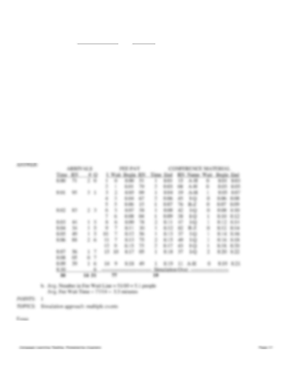
Chapter 12 – Simulation
to the following distribution:
Number of Arrivals Probability
0 .30
1 .30
2 .30
3 .10
The time to pay one’s fees is either one minute or two minutes depending upon whether one uses a check or credit card.
The probability of a one-minute time is .60.
After paying his fees, an attendee then goes to the correct line for the conference materials. At this year’s conference 35%
of the attendees have last names beginning with A-H, 36% with last names beginning with I-Q, and 29% with last names
beginning with R-Z. The time required to pick up conference materials is fixed at 2 minutes.
a. Simulate the waiting line for the first 10 minutes of the morning registration that begins at 8:00 AM. Use the
following random numbers to generate:
Number of arrivals in any given minute: 71, 95, 83, 44, 34, 49, 88, 56, 05, 39
Registration fee service time: 51, 79, 09, 67, 15, 58, 04, 78, 30, 56
First letter of the last name: 15, 08, 19, 45, 76, 42, 38, 47, 82, 37
b. What is the average size of the waiting line to pay fees (not including the person being served), and the average
customer waiting time to pay fees based on this simulation?
b. Avg. Number in Fee Wait Line = 51/10 = 5.1 people
Simulation approach: multiple events
57. Simulation is to be used to study customer waiting patterns at several branches of an organization. Acknowledging
that arrivals and service times follow different distributions over the branches, of what use is the development of a
Chapter 12 – Simulation
general simulation model?
58. Why would one want to use a general purpose programming language rather than a spreadsheet to develop a
simulation?
59. How are both analysts and managers involved in the validation process?
60. How can historical information be used to create discrete probability distributions?
61. Why is a flowchart useful in simulation?
62. Explain the difference between verification and validation as they relate to a simulation model.