21
Copyright © 2019 Pearson Education, Inc.
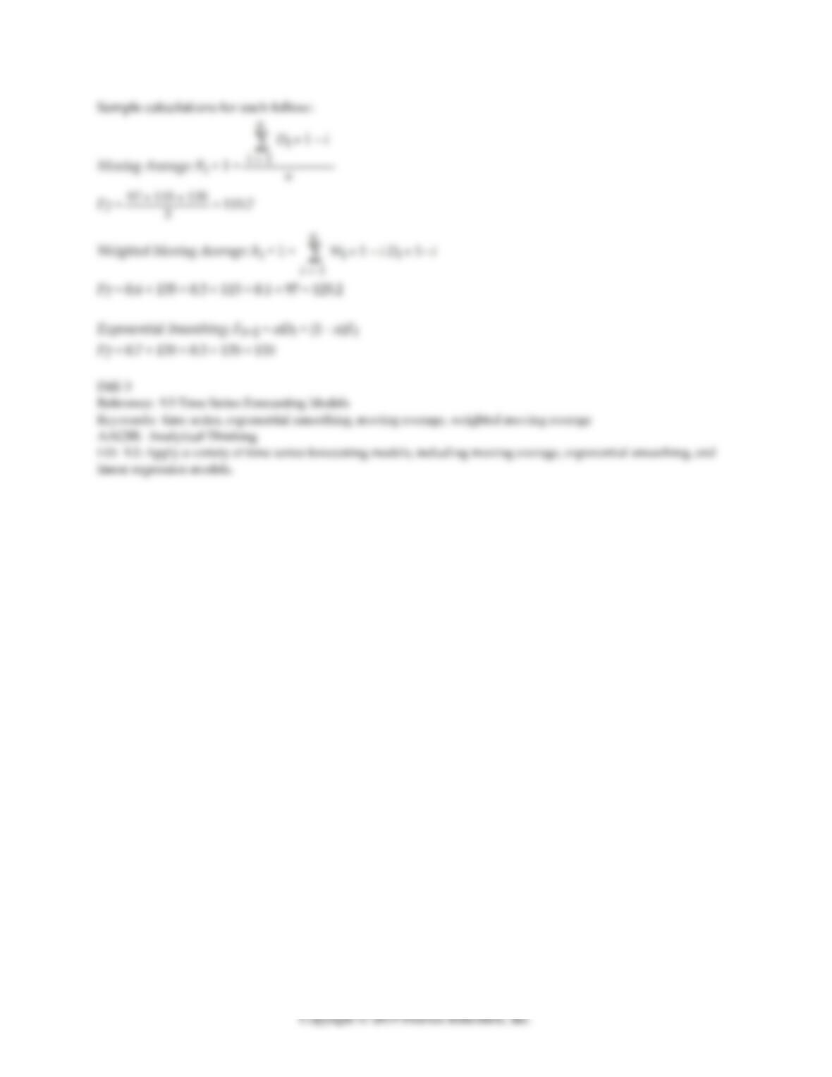
Sample calculations for each follow:
Moving Average: Ft + 1 =
F7 = = 115.7
Weighted Moving Average: Ft + 1 =
F7 = 0.6 × 135 + 0.3 × 115 + 0.1 × 97 = 125.2
Exponential Smoothing: Ft+1 = αDt + (1 – α)Ft
F7 = 0.7 × 135 + 0.3 × 135 = 135
Diff: 3
Reference: 9.5 Time Series Forecasting Models
Keywords: time series, exponential smoothing, moving average, weighted moving average
AACSB: Analytical Thinking
LO: 9.2: Apply a variety of time series forecasting models, including moving average, exponential smoothing, and
linear regression models.
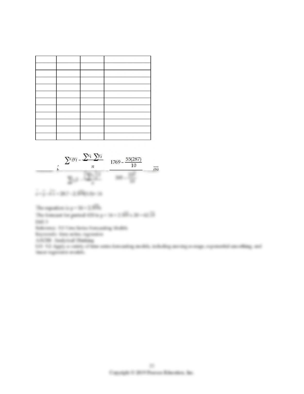
31) Using the data shown in the table, develop a regression line that can be used to predict the demand
for time period number 20. What is the regression equation and what is your forecast for period 20?
Period
Demand
Period ∗ Demand
1
16
16
2
20
40
3
24
72
4
27
108
5
29
145
6
30
180
7
32
224
8
35
280
9
36
324
10
38
380
Sums
55
287
1769
23
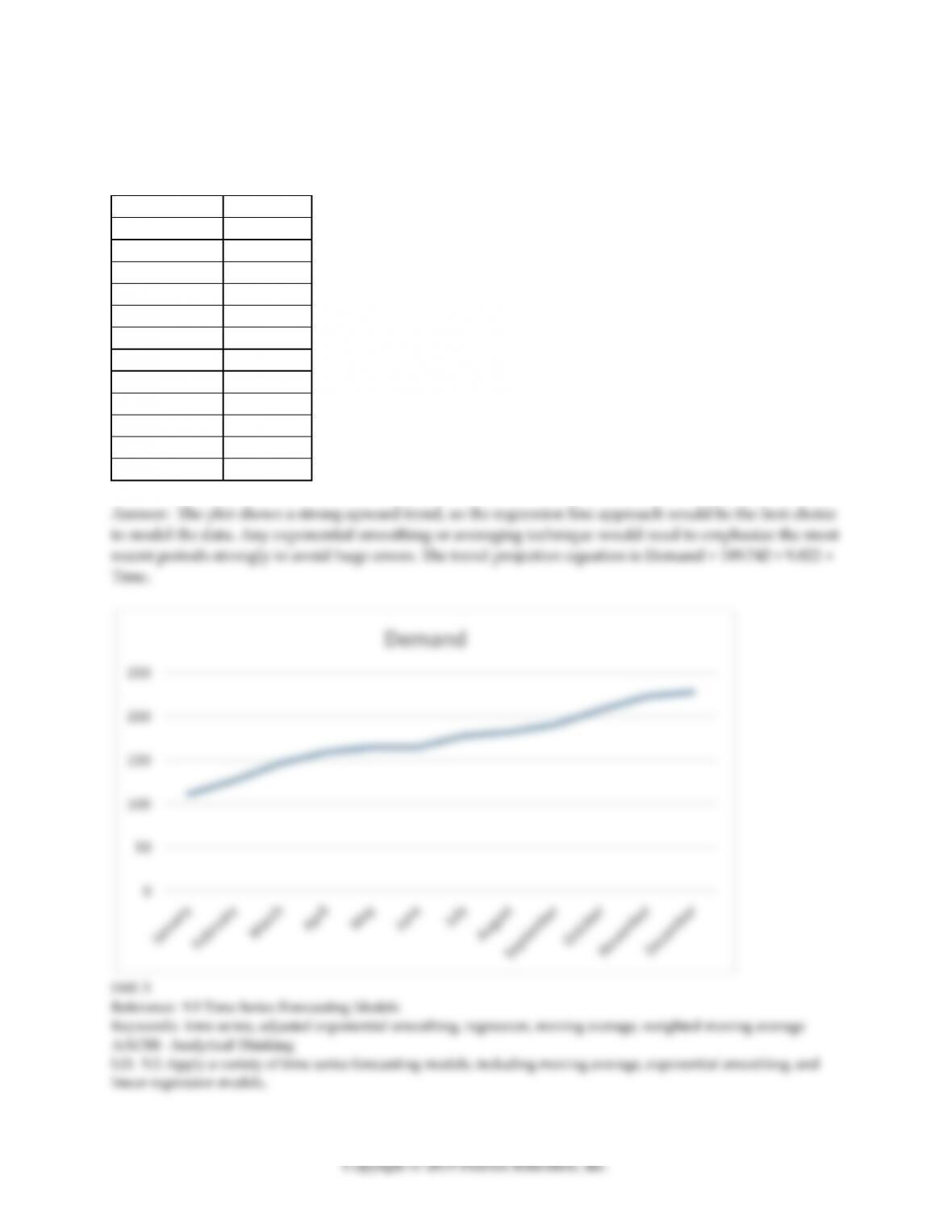
32) A counseling service records the number of calls to their hotline for the last year. Plot the data and
determine which forecasting technique would be best among a moving average, weighted moving
average, exponential smoothing, and regression line.
Month
Demand
January
111
February
127
March
146
April
159
May
165
June
165
July
178
August
182
September
191
October
208
November
223
December
228
33) The Pancake House did a brisk business on the weekend and the maître d’ was always on the lookout
for ways to improve the customer experience. He carefully tracked the number of customers that graced
their establishment over the last four weekends. He was hopeful that he could forecast the number of
customers that would come for the world‘s finest pancakes the next weekend.
Weekend 1
Weekend 2
Weekend 3
Weekend 4
Friday
131
216
286
355
Saturday
225
311
408
490
Sunday
166
249
330
415
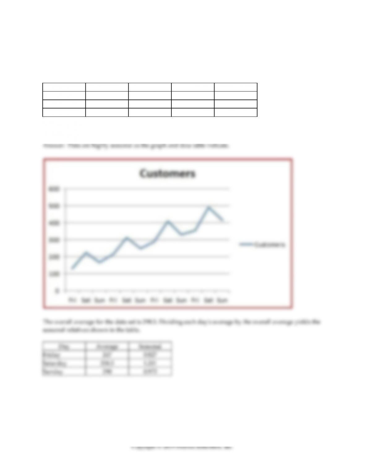
Using the data in the table, first plot the data and comment on the appearance of the demand pattern.
Then develop a forecast for weekend #5 that fits the data.
Friday
247
Saturday
Sunday
290
25
Copyright © 2019 Pearson Education, Inc.
Divide each entry in the table by the seasonal relative. Use linear regression with the first Friday as 1 and
the last Sunday as 12 to yield the regression equation
Customers = 122.8 + 27.03 ∗ Day #
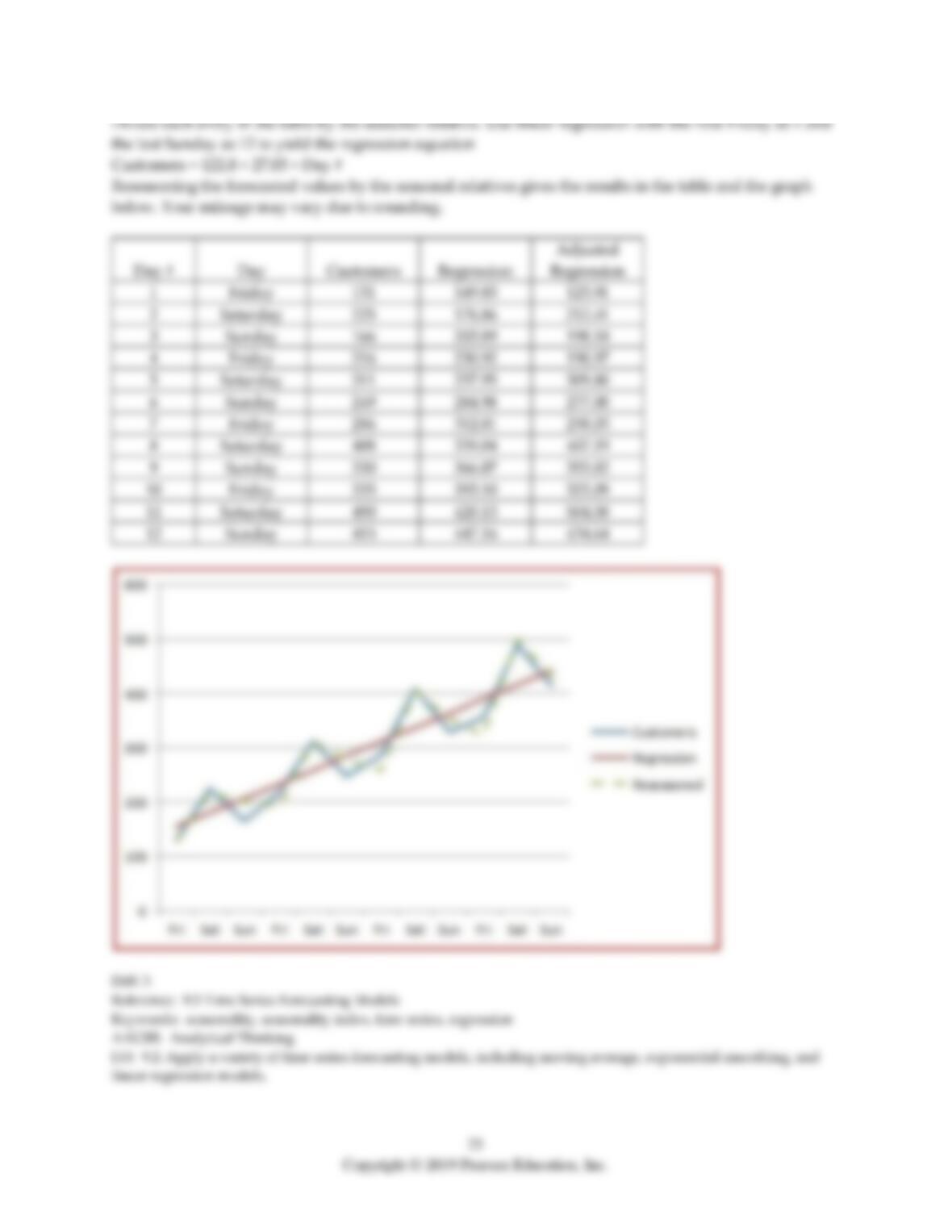
Reseasoning the forecasted values by the seasonal relatives gives the results in the table and the graph
below. Your mileage may vary due to rounding.
Day #
Day
Customers
Regression
Adjusted
Regression
1
Friday
131
149.83
123.91
2
Saturday
225
176.86
212.41
3
Sunday
166
203.89
198.18
4
Friday
216
230.92
190.97
5
Saturday
311
257.95
309.80
6
Sunday
249
284.98
277.00
7
Friday
286
312.01
258.03
8
Saturday
408
339.04
407.19
9
Sunday
330
366.07
355.82
10
Friday
355
393.10
325.09
11
Saturday
490
420.13
504.58
12
Sunday
415
447.16
434.64
Diff: 3
Reference: 9.5 Time Series Forecasting Models
Keywords: seasonality, seasonality index, time series, regression
AACSB: Analytical Thinking
LO: 9.2: Apply a variety of time series forecasting models, including moving average, exponential smoothing, and
linear regression models.
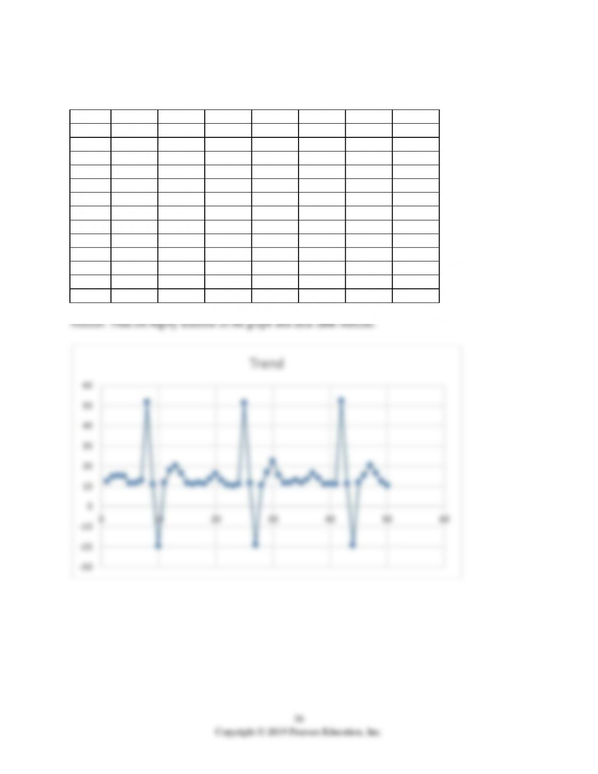
34) Using the data in the table, first plot the data and comment on the appearance of the demand pattern.
Then develop a forecast for periods 51-70 that fits the data.
Time
Output
Time
Output
Time
Output
Time
Output
1
12.5
14
16.4
27
-19.2
40
11.3
2
14.8
15
11.7
28
10.6
41
11.1
3
15.3
16
11.1
29
16.8
42
52.5
4
15
17
11.9
30
22.5
43
11.3
5
11.5
18
11.3
31
15.5
44
-19.3
6
11.6
19
13.7
32
11.7
45
12
7
12.8
20
16.3
33
11.9
46
15.5
8
51.9
21
13.1
34
13
47
20.5
9
11
22
10.8
35
11.9
48
16.5
10
-19.7
23
10.3
36
13.5
49
12.5
11
11.9
24
11
37
16.5
50
10.5
12
17.8
25
51.4
38
14
13
20.3
26
11.6
39
11
27
Copyright © 2019 Pearson Education, Inc.
Peaks near 50 occur at points 8, 25 and 42, and this seasonality is reflected in the other significant features
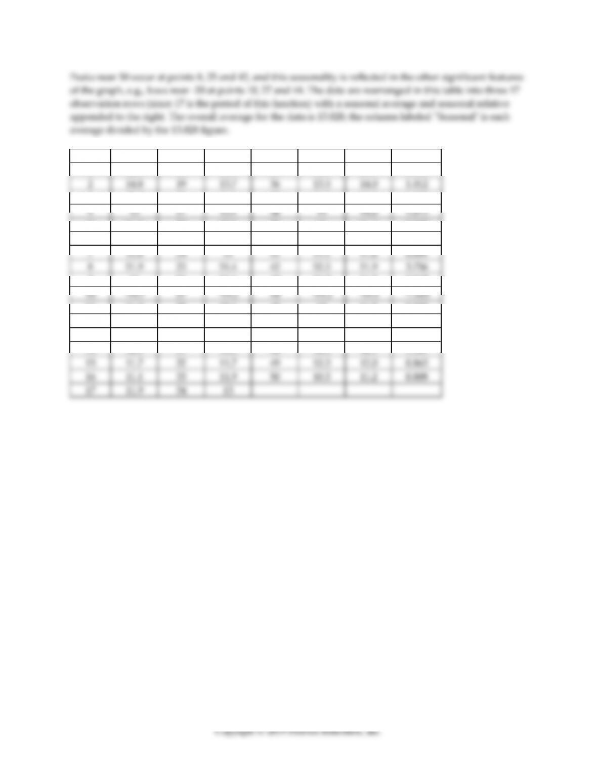
of the graph, e.g., lows near -20 at points 10, 27 and 44. The data are rearranged in this table into three 17
observation rows (since 17 is the period of this function) with a seasonal average and seasonal relative
appended to the right. The overall average for the data is 13.828; the column labeled “Seasonal” is each
average divided by the 13.828 figure.
Time
Output
Time
Output
Time
Output
Average
Seasonal
1
12.5
18
11.3
35
11.9
11.9
0.861
2
14.8
19
13.7
36
13.5
14.0
1.012
3
15.3
20
16.3
37
16.5
16.0
1.159
4
15
21
13.1
38
14
14.0
1.015
5
11.5
22
10.8
39
11
11.1
0.803
6
11.6
23
10.3
40
11.3
11.1
0.800
7
12.8
24
11
41
11.1
11.6
0.841
8
51.9
25
51.4
42
52.5
51.9
3.756
9
11
26
11.6
43
11.3
11.3
0.817
10
-19.7
27
-19.2
44
-19.3
-19.4
-1.403
11
11.9
28
10.6
45
12
11.5
0.832
12
17.8
29
16.8
46
15.5
16.7
1.208
13
20.3
30
22.5
47
20.5
21.1
1.526
14
16.4
31
15.5
48
16.5
16.1
1.167
15
11.7
32
11.7
49
12.5
12.0
0.865
16
11.1
33
11.9
50
10.5
11.2
0.808
17
11.9
34
13
28
Copyright © 2019 Pearson Education, Inc.
Divide each entry in the table by the seasonal relative. Then use linear regression with independent
variables ranging from 1-50 to yield the regression equation
Output = 14.05629-0.00895 ∗ Time
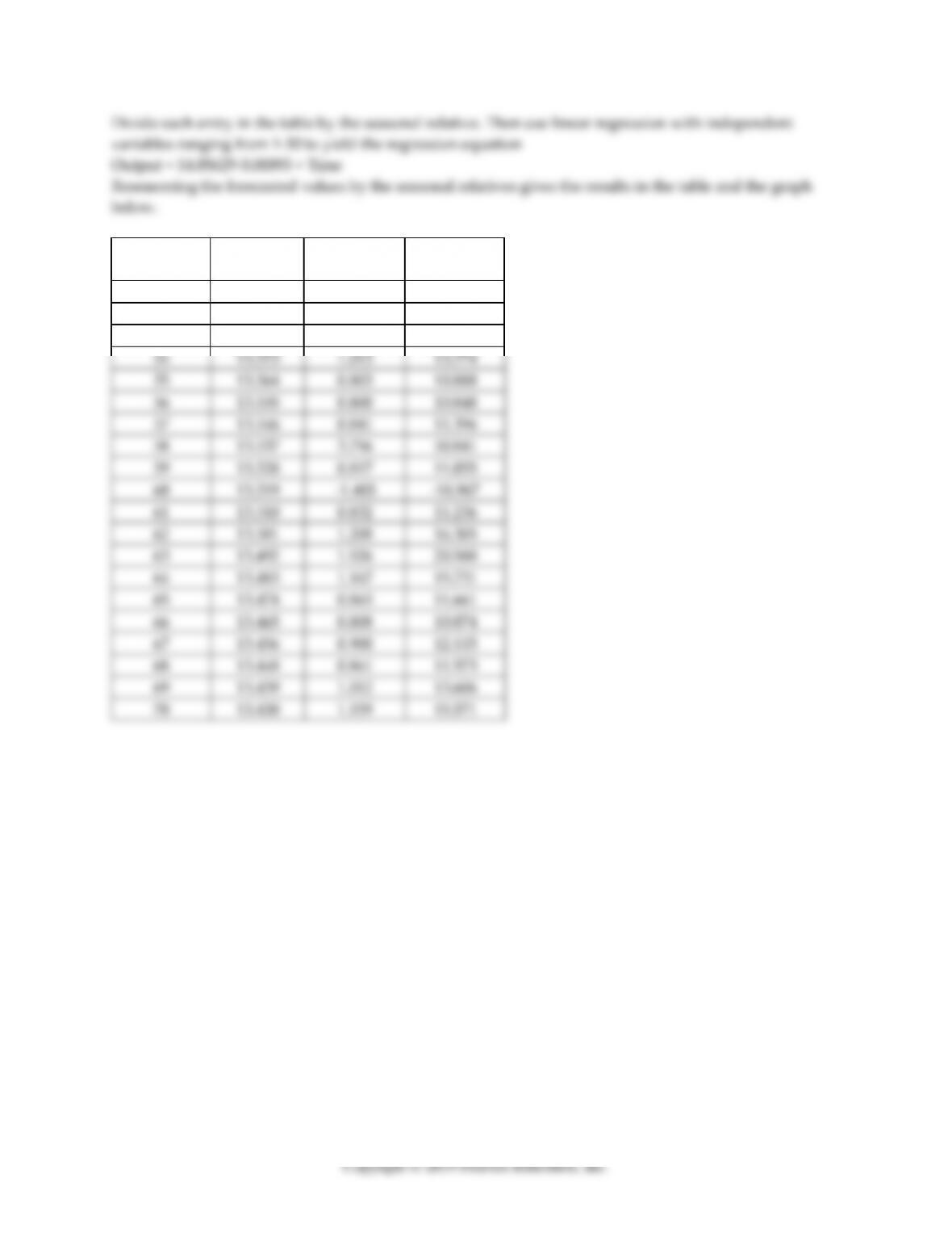
Reseasoning the forecasted values by the seasonal relatives gives the results in the table and the graph
below.
Time
Regression
Index
Seasonally
Adjusted
51
13.600
0.861
11.704
52
13.591
1.012
13.760
53
13.582
1.159
15.748
54
13.573
1.015
13.774
55
13.564
0.803
10.888
56
13.555
0.800
10.848
57
13.546
0.841
11.396
58
13.537
3.756
50.841
59
13.528
0.817
11.055
60
13.519
-1.403
-18.967
61
13.510
0.832
11.236
62
13.501
1.208
16.305
63
13.492
1.526
20.588
64
13.483
1.167
15.731
65
13.474
0.865
11.661
66
13.465
0.808
10.874
67
13.456
0.900
12.115
68
13.448
0.861
11.573
69
13.439
1.012
13.606
70
13.430
1.159
15.571
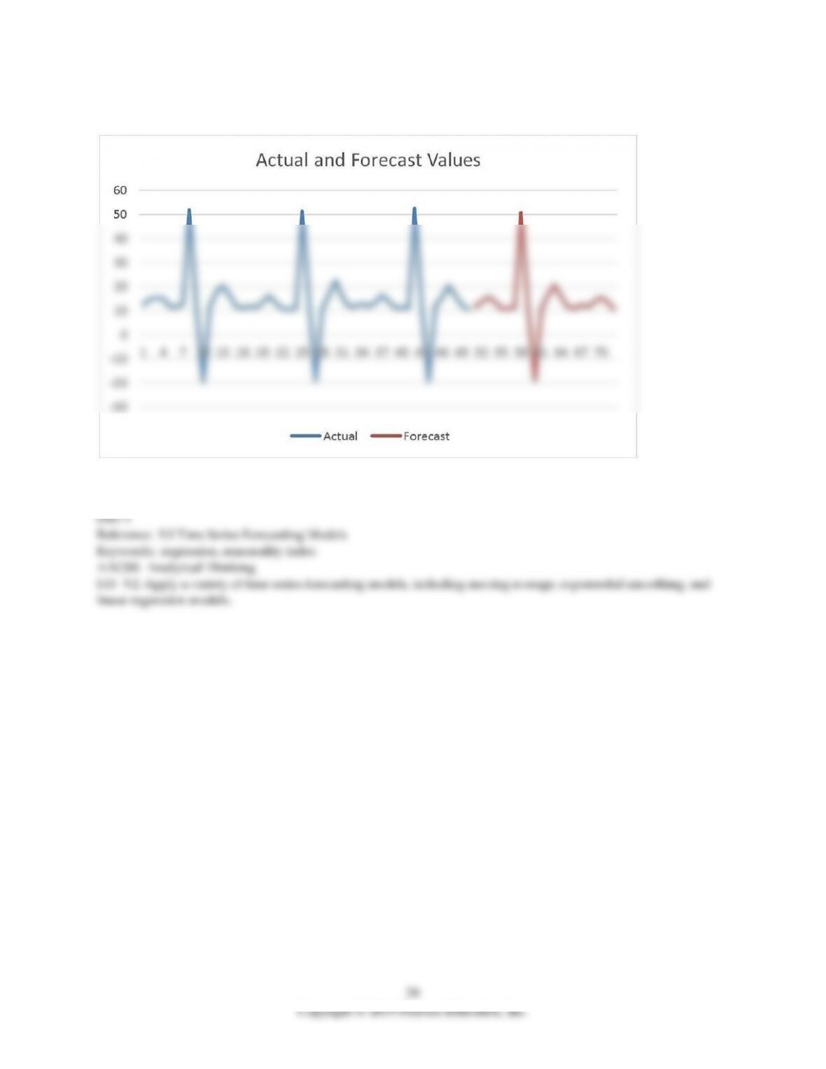
The graph below is a plot of the original data for points 1–50 and the forecast points 51–70.
9.6 Casual Forecasting Models
1) A well-educated lumberjack decides to use linear regression to predict the demand for firewood based
on the ambient temperature. He has collected data on firewood sales and temperature for the last several
days and has performed some preliminary calculations as shown in the table. What is his regression
equation based on the data?
Temp
Ricks
Temp Squared
Temp ∗ # Ricks
33
17
1089
561
19
32
361
608
34
20
1156
680
34
18
1156
612
20
33
400
660
24
30
576
720
17
34
289
578
30
25
900
750
38
16
1444
608
23
29
529
667
Sums
272
254
7900
6444
A) Ricks = 50.6 – 0.93 × Temp
B) Temp = 53.3 – 1.0 × Ricks
C) Ricks = 0.93 – 50.6 × Temp
D) Temp = 1.0 – 53.3 × Ricks
31
2) A poultry farmer that dabbles in statistics is interested in exploring the relationship between two types
of feed (layer pellets and scratch), water, and the output of his laying hens. For ten days he records the
number of ounces of layer pellets and scratch the hens consume and the number of fluid ounces of water
and tracks the number of eggs that are produced. What is his regression equation based on the data?
Scratch
Layer Pellets
Water
Eggs
48
29
36
24
44
27
34
22
41
22
31
20
42
21
32
20
48
23
34
22
44
28
34
23
42
22
37
21
41
28
33
22
42
22
31
20
47
29
37
24
A) Eggs = 6.56 + .38Scratch + .17Pellets + .21Water
B) Eggs = 1.25 + .18Scratch + .29Pellets + .15Water
C) Eggs = 0.93 – .88Scratch + .37Pellets + .41Water
D) Eggs = 4.22 + .37Scratch + .67Pellets + .58Water
32
3) A poultry farmer that dabbles in statistics is interested in exploring the relationship between layer
pellets and the output of his laying hens. For ten days he records the number of ounces of layer pellets
and the number of eggs that are produced. What is his regression equation based on the data?
Layer Pellets
Eggs
29
24
27
22
22
20
21
20
23
22
28
23
22
21
28
22
22
20
29
24
A) Eggs = 11.3 + 0.42Pellets
B) Eggs = 1.25 + 0.29Pellets
C) Eggs = 10.9 + 0.23Pellets
D) Eggs = 4.22 + 0.67Pellets
33
4) A poultry farmer that dabbles in statistics is interested in exploring the relationship between two types
of feed (layer pellets and scratch), water, and the output of his laying hens. For ten days he records the
number of ounces of layer pellets and scratch the hens consume and the number of fluid ounces of water
and tracks the number of eggs that are produced. After running a multiple regression model, he obtains
the following report. What is the best interpretation of these statistics?
Regression Statistics
Multiple R
0.993633
R Square
0.987307
Adjusted R Square
0.98096
Standard Error
0.213764
Observations
10
A) The probability that the number of eggs is correctly predicted by the amount of scratch, layer pellets,
and water consumed is 99.36%.
B) The prediction of the amount of eggs is 98.7% accurate based on the amount of scratch, layer pellets,
and water consumed.
C) 98.7% of the variability in egg production is explained by the amount of water, scratch, and layer
pellets consumed.
D) The prediction of the amount of eggs is 99.36% accurate based on the amount of scratch, layer pellets,
and water consumed.
34
5) A poultry farmer that dabbles in statistics is interested in exploring the relationship between two types
of feed (layer pellets and scratch), water, and the output of his laying hens. For ten days he records the
number of ounces of layer pellets and scratch the hens consume and the number of fluid ounces of water
and tracks the number of eggs that are produced. After running a multiple regression model, he obtains
the following report. What is the best interpretation of these statistics?
Coefficients
Std Error
t Stat
P-value
Intercept
1.256
1.249
1.006
0.353
Scratch
0.185
0.032
5.714
0.001
Layer Pellets
0.295
0.026
11.539
0.000
Water
0.149
0.041
3.587
0.012
A) For every egg produced, about 0.185 ounces of scratch must be consumed.
B) The standard error for the model intercept is as large as the coefficient, thus the intercept is the most
important predictor of egg production.
C) Layer pellets are not good predictors of egg production because the p-value is 0.
D) For every ounce of water consumed, the chickens produce 0.15 eggs, holding all other independent
variables constant.
6) McMahon and Tate advertising company is interested in an appropriate mix of print, radio, and
television ads for their new client. Darrin Stevens performs a multiple regression on the effects of dollars
spent on each type of media on dollars of sales of product. Darrin uses data from the most recent
advertising campaigns and develops the following equation:
y = 254,215 + 6.79 × Print – 1.4 × Radio + 16.87 × Television
The r-squared statistic is 0.77 and all coefficients are significant. Which of the following statements is
best?
A) At a minimum, the client will sell $254,215 worth of product after the new advertising campaign.
B) At a maximum, the client will sell $254,215 worth of product after the new advertising campaign.
C) This equation will be of no use in predicting the amount of sales based on advertising in these media.
D) The client should spend more money on television advertising than on radio advertising.
35
7) Which of these quantitative techniques can be a causal model?
A) linear regression
B) last period
C) exponential smoothing
D) weighted moving average
8) Heidi runs a multiple regression for the output of cheese curds by using the daily temperature and the
consumption of sweet clover. The intercept term is 23, the slope coefficient for the daily temperature is 1.5
and the slope coefficient for the consumption of sweet clover is 0; both coefficients are statistically
significant. Which of these conclusions is most appropriate?
A) Heidi should collect more data.
B) The most important term in Heidi’s model is the intercept.
C) As the daily temperature rises, the intercept term probably decreases.
D) Heidi should drop the sweet clover term from her model.
9) As yet another earthquake rattled her china cabinet, the data scientist decided to test whether
hydraulic fracturing (where water is injected into the Earth) truly was predictive of the number of
earthquakes in the region. What is the slope of the regression equation based on the data?
Injections
Earthquakes
137
682
331
833
360
905
442
1008
478
1482
529
1742
A) 151.24
B) 2.52
C) 0.85
D) 0.72