CHAPTER 3
APPLICATIONS OF LINEAR AND INTEGER PROGRAMMING MODELS
TRUE/FALSE QUESTIONS
1. It takes two pounds of steel and three pounds of copper to
make a particular product. If there are 100 pounds of steel and 100
pounds of cooper available, one constraint will be 2X1 + 3X2 200.
2. You are currently paying $12 per hour for labor, and labor
costs are included in the calculation of the objective function
coefficients of a maximization problem. The shadow price for labor
printed on the sensitivity analysis report is $8. It would be
economically beneficial to you if you could secure extra labor for
3. The objective function coefficient for X1 is currently $18 and
for X2 is $29, and the ranges of optimality for these coefficients
are between $15 and $20 and between $25 and $35, respectively. If
the objective function coefficients for X1 and X2 decline by $2 each,
since both coefficients are still within their ranges of optimality,
4. A linear programming model has a constraint that reflects a
budget restriction of $100,000. The range of feasibility for this
amount, reflected on the sensitivity report, is $85,000 to $325,000.
Thus if the budget restriction is changed to $90,000, the optimal
5. Nimble Automotive uses linear programming to produce a monthly
production schedule for their manufacturing plant. Although the
number of cars built is obviously an integer, the fractional part of
a non-integer decision variable could be considered “work in
6. If project 1 is performed then project 2 will not be
performed. This can be modeled by the constraint X1 – X2 1, where
7. One approach for solving an integer linear programming problem
is simply to enumerate all feasible points and select the one
yielding the “best” value for the objective function. However, the
number of feasible integer points is usually so large, even for
small problems, that this approach is inefficient for solving most
8. The optimal solution obtained to a maximization integer linear
programming model, where the integer requirements are at first
ignored, provides a lower bound for the optimal objective function
9. Relaxing the integer restrictions to an integer linear model
produces an optimal solution of X1 = 23 and X2 = 15. This must also
10. In a fixed charge integer linear model where there are
variable profits of $45 and $80 for producing products 1 and 2, and
a fixed charge of $1000 if any of product 2 is produced, the
objective function can be modeled by MAX 45X1 + 80X2 – 1000Y2, where
11. If at most 3 of 7 projects are to be performed, this can be
modeled by X1 + X2 + X3 + X4 + X5 + X6 + X7 3, where X1, X2, X3, X4,
X5, X6, and X7 are all restricted to be non–negative, have an upper
12. Joe Chan is modeling the installation of smoke alarms. The
constraint Y1 – Y2 0 uses the binary variables Y1 for upstairs
installation and Y2 for downstairs installation. The constraint
implies that if the first installation is performed, the second must
13. A maximization integer linear model is solved by first
relaxing the integer restrictions, giving an optimal solution to the
resulting linear model of X1 = 6, X2 = 11. The shadow price for the
first constraint is $9, and the range of feasibility has a maximum
increase of 20 and a maximum decrease of 5. Then for the integer
model, X1 = 6, X2 = 11 is the optimal solution. If there is an
increase of 3 units of the first resource, the optimal value of the
14. A management science professional with extensive modeling
experience will focus on management concerns and need not spend much
15. The optimal solution to a supply chain management model can be
found by solving the standalone separate components of the process.
MULTIPLE CHOICE QUESTIONS
1. The shadow price for a constraint that expresses that the
availability of wood is 3000 board-feet is $0.50, and the range of
feasibility is between 2800 and 4000 board-feet. Which of the
following is not correct?
a. All 3000 board-feet of wood will be used.
b. If only 2900 board-feet of wood are available, the
optimal objective function value will be reduced by $50.
c. If only 2900 board-feet of wood are available, the
optimal solution will not change.
d. If 6000 board-feet of wood are available, the objective
function value will increase by at least $500.
2. Hong Securities has $300,000 to invest in four stocks and
three bonds. X1, X2, X3, and X4 denote the amounts invested in each
of the stocks, and Y1, Y2, and Y3 equal the amounts invested in each
of the three bonds. Which of the following shows that at least 40%
of the investment in stocks must be in stock 1?
a. X1 120,000
b. X1 – .4X2 –.4X3 – .4X4 0
c. .6X1 – .4X2 – .4X3 – .4X4 0
d. X1 .4(X2 + X3 + X4 + Y1 + Y2 + Y3)
3. In problem 2, let A = the total amount invested in stocks and
B = the total amount invested in bonds. To state that at least 40%
of the investment in stocks must be in stock 1, two constraints in
the model would be:
a. X1 – .4A 0, X2 + X3 + X4 – A = 0
b. X1 – .4A 0, X1 + X2 + X3 + X4 – A = 0
c. X1 – .4A – .4B 0, A + B = 300,000
d. X1 – .4A – .4B 0, A + B = 300,000
4. Which of the following is true when using summation variables?
a. The number of constraints will stay the same as in a
formulation without the use of summation variables.
b. The number of variables will stay the same as in a
formulation without the use of summation variables.
c. There are typically fewer non-zero input coefficients on
the left side of the constraints.
d. Percentage constraints cannot be formulated without the
use of summation variables.
5. The optimal solution value of an integer linear programming
problem with a minimization objective function may not be __________
the optimal solution value if integer requirements are ignored.
a. the same as
b. less than
c. greater than
d. a rounded form of
6. Nike will build a factory at Millville or Greenfield, but not
both. Alternatively, Nike may choose to build at neither location.
The appropriate linear constraint to express this restriction using
binary variables Y1 and Y2 is:
a. Y1 – Y2 1
b. Y1 + Y2 1
c. Y1 + Y2 = 1
d. Y1 – Y2 0
7. Nike must build a factory at either Millville or Greenfield,
but not both. The appropriate linear constraint to express this
restriction using binary variables Y1 and Y2 is:
a. Y1 – Y2 1
b. Y1 + Y2 1
c. Y1 + Y2 = 1
d. Y1 – Y2 0
8. Nike may build a factory at Millville (Y1) or it may not. It
may also build a regional warehouse at the same site (W1). But Nike
will not build a warehouse without also building a factory. So, its
choices are: (1) neither factory nor warehouse; (2) factory only;
or (3) factory and warehouse. The appropriate linear constraint to
express this is:
a. Y1 – W1 1
b. Y1 + W1 1
c. Y1 + W1 0
d. Y1 – W1 0
9. Billyboy Toys’ toy balls, bats, and gloves net profits,
excluding fixed costs, of $7, $8, and $13 respectively. The
products require 2, 3, and 5 production hours each. Using current
facilities, 1600 production hours are available for the production
of these products each month. If Billyboy also leases a second,
smaller production facility for $3000 per month, this will increase
the availability of production hours for these products by 800.

This situation can be modeled using a mixed integer model that
includes the following:
a. An objective function of: MAX 7X1 + 8X2 + 13X3
Constraints including: 2X1 + 3X2 + 5X3 2400
Variable constraints including X1, X2, X3 0
b. An objective function of: MAX 7X1 + 8X2 + 13X3 – 3000Y1
Constraints including: 2X1 + 3X2 + 5X3 – 800Y1 2400
Variable constraints including X1, X2, X3 0, Y1 = 0 or 1
c. An objective function of: MAX 7X1 + 8X2 + 13X3 – 3000Y1
Constraints including: 2X1 + 3X2 + 5X3 + 800Y1 1600
Variable constraints including X1, X2, X3 0, Y1 = 0 or 1
d. An objective function of: MAX 7X1 + 8X2 + 13X3 – 3000Y1
Constraints including: 2X1 + 3X2 + 5X3 – 800Y1 1600
Variable constraints including X1, X2, X3 0, Y1 = 0 or 1
10. Two constraints in a model with binary variables Y1, Y2, Y3
representing whether or not project 1, 2, or 3 will be performed
are: Y1 – Y2 0 and Y1 – Y3 0. Taken together, what can be
inferred from these constraints?
a. Projects 2 and 3 cannot both be performed.
b. Projects 2 and 3 must be performed if project 1 is
performed.
c. Projects 2 and 3 may be performed is project is
performed.
d. Project 1 must be performed.
11. You have formulated a problem with three constraints: (1) 2X1
+ 3X2 + 4X3 300; (2) X1 + X2 40; (3) X1 + X2 + X3 = 100. Which of
the following states that at least 2 of these 3 constraints must
hold? (M = a large value)
a. 2X1 + 3X2 + 4X3 – MY1 300
X1 + X2 – MY2 40
X1 + X2 + X3 – MY3 = 100
Y1 + Y2 + Y3 2
b. 2X1 + 3X2 + 4X3 – MY1 300
X1 + X2 – MY2 40
X1 + X2 + X3 + MY3 100
Y1 + Y2 + Y3 2
c. 2X1 + 3X2 + 4X3 – MY1 300
X1 + X2 + MY2 40
X1 + X2 + X3 – MY3 100
X1 + X2 + X3 + MY3 100
Y1 + Y2 + Y3 1
d. 2X1 + 3X2 + 4X3 – MY1 300
X1 + X2 – MY2 40
X1 + X2 + X3 – MY3 100
Y1 + Y2 + Y3 1
12. What is the initial step in the process of building linear
models?
a. Define the constraints.
b. Graph the problem.
c. Determine decision variables.
d. Make sure a feasible solution exists.
13. Review this Excel spreadsheet:
Based on the figures in the spreadsheet, we can conclude:
a. Atlantic Lighting is included in the optimal result.
b. Atlantic Lighting would be included in the optimal
result if its objective coefficient were 20.333.
c. The range of optimality for Bedrock Insurance is 19.57
to 20.5.
d. The range of feasibility for the total expected return
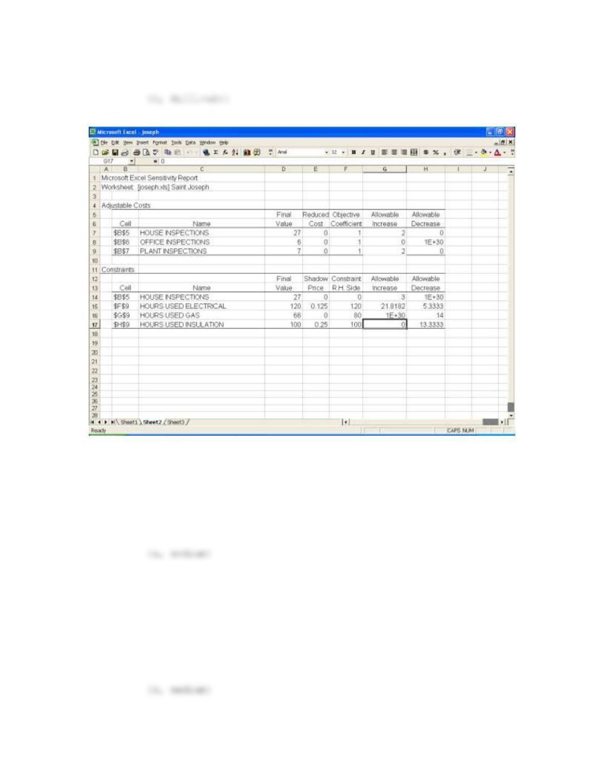
is 6980 to 7880.
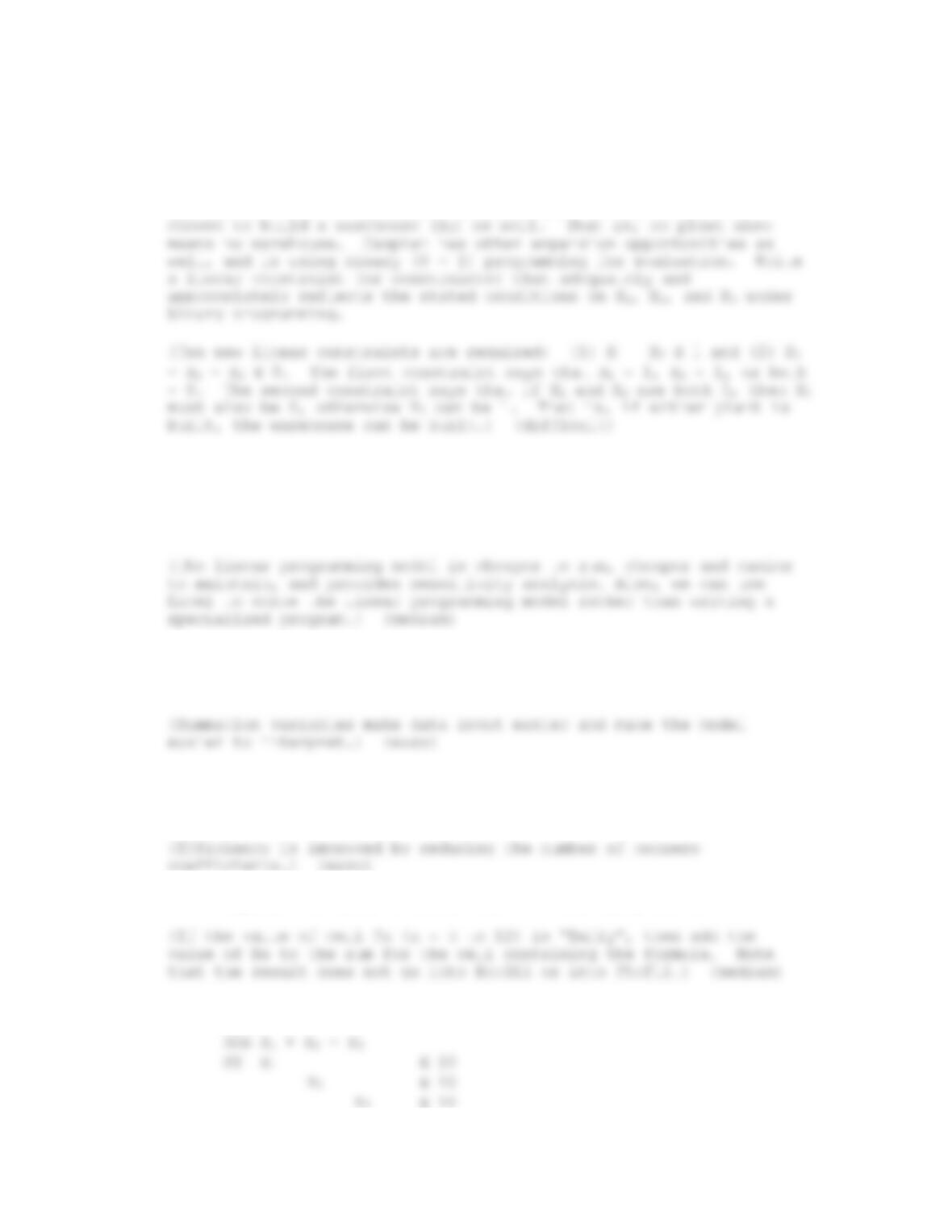
14. Review the Excel spreadsheet below.
Based on the information in the spreadsheet, we can conclude:
a. There may be alternate optimal solutions.
b. The range of feasibility for Hours Used Electrical is
unlimited.
c. For every extra unit of Hours Used Gas, the objective
function value will increase by 80.
d. The range of optimality for House Inspections is 25 to
29.
15. Silver’s Gym offers Kickboxing I, Kickboxing II, and
Kickboxing III, and Ms. DeVore insists on teaching all three
classes. Otherwise, the gym will offer no kickboxing classes. How
would you model this constraint?
a. X1 + X2 + X3 = 0
b. X1 + X2 + X3 = 3
c. X1 + X2 + X3 0
d. X1 – X2 = 0 and X1 – X3 = 0

16. What is Data Envelopment Analysis?
a. A linear programming based approach to determine the
relative efficiency of entities with similar goals and
objectives.
b. A decision support system that envelops the entire
manufacturing and shipping process into an integrated
system.
c. An integer linear programming technique involving
solving a series of linear programming models and using
the solutions as bounds on the integer solution.
d. A form of sensitivity analysis that allows the
simultaneous changing of multiple decision variable
values.
17. XLB Sports has 30 franchises (teams). Although most of the
teams make an annual profit, some teams report losses. An owner of
a team that loses money can still make a profit when he sells the
franchise since equity increases have been greater than reported
losses. XLB has requested a model to determine which, if any,
franchises should be eliminated. The costs associated with team
elimination include the buyout of the owner, paying off existing
contracts such as ballpark leases, and anticipated legal costs. The
objective function is the overall profit of XLB. Because all teams
must play on the same day, the number of teams must be an even
number. Some teams may lose money at home but help other teams by
drawing well in road games.
Which of the following is true?
a. Teams reporting a loss should be eliminated.
b. You should use binary variables in a mixed integer
model.
c. The problem can be solved by solving 30 team integer
linear programming models.
d. The problem cannot be modeled.
SHORT ANSWER QUESTIONS
1. Caspian Seafoods has recently purchased a very large property
for possible expansion of its business. On this property, Caspian
may construct a large plant (X1) or a small plant (X2). In addition,
if, and only if, it constructs either plant, it may or may not
2. Marc Leaser, who has a PhD from MIT, has created a process
model using first and second order differential equations. He
correctly points out that your linear programming model of the same
process makes significant simplifying assumptions which make the
linear solution suboptimal. What is your reply to management?
3. Why use summation variables, which make the linear programming
model larger? The model can be completed without summation
variables.
4. Adding a constraint increases the time needed to solve a
linear programming model. Why then might adding a summation
variable actually improve model efficiency?
5. Explain the Excel formula SUMIF(F5:F12,”Daily”,B5:B12).
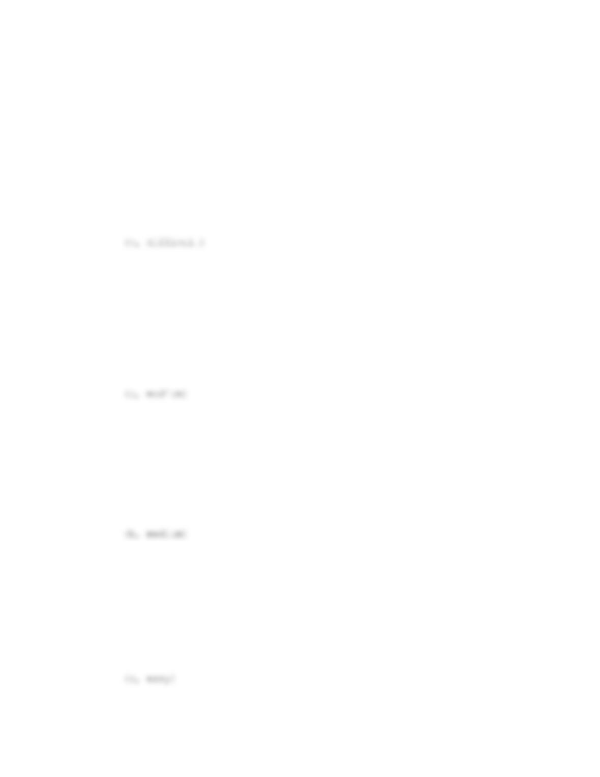
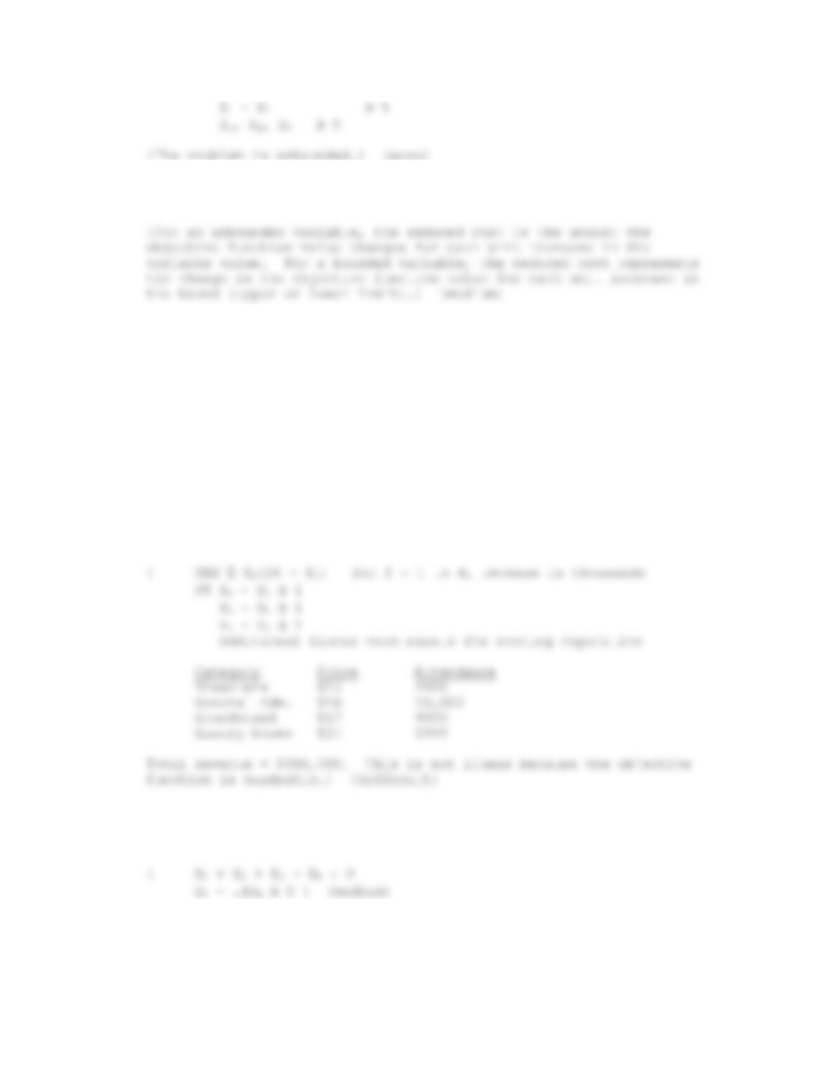
6. What is wrong with this model?
7. What is the difference in the interpretation of reduced cost
for an unbounded variable versus a bounded variable?
8. The availability of seats for ballgames at Oliver Field is
Bleachers 4000 seats A1
General Admission 10,000 seats A2
Grandstand 10,000 seats A3
Luxury Boxes 1000 seats A4
A1 through A4 represent the attendance in the different seating
options at prices X1, X2, X3, and X4. Better seats must cost at least
$1 more than the next lower category. If the team charges $1 per
seat, the demand will be 25,000. For each $1 increase in ticket
price, the demand drops by 1000. The team owner has set up an
integer programming model to maximize revenue (not necessarily to
sell out).
What prices should be charged? Is this a linear programming model?
9. X1 is limited to 40% of the total, as modeled by the constraint
.6X1 – .4X2 – .4X3 0. Rewrite this as two constraints using a
summation variable.
10. Why use hidden cells in an Excel spreadsheet representation of
a linear programming model?

FORMULATION/SOLUTION/ANALYSIS QUESTIONS
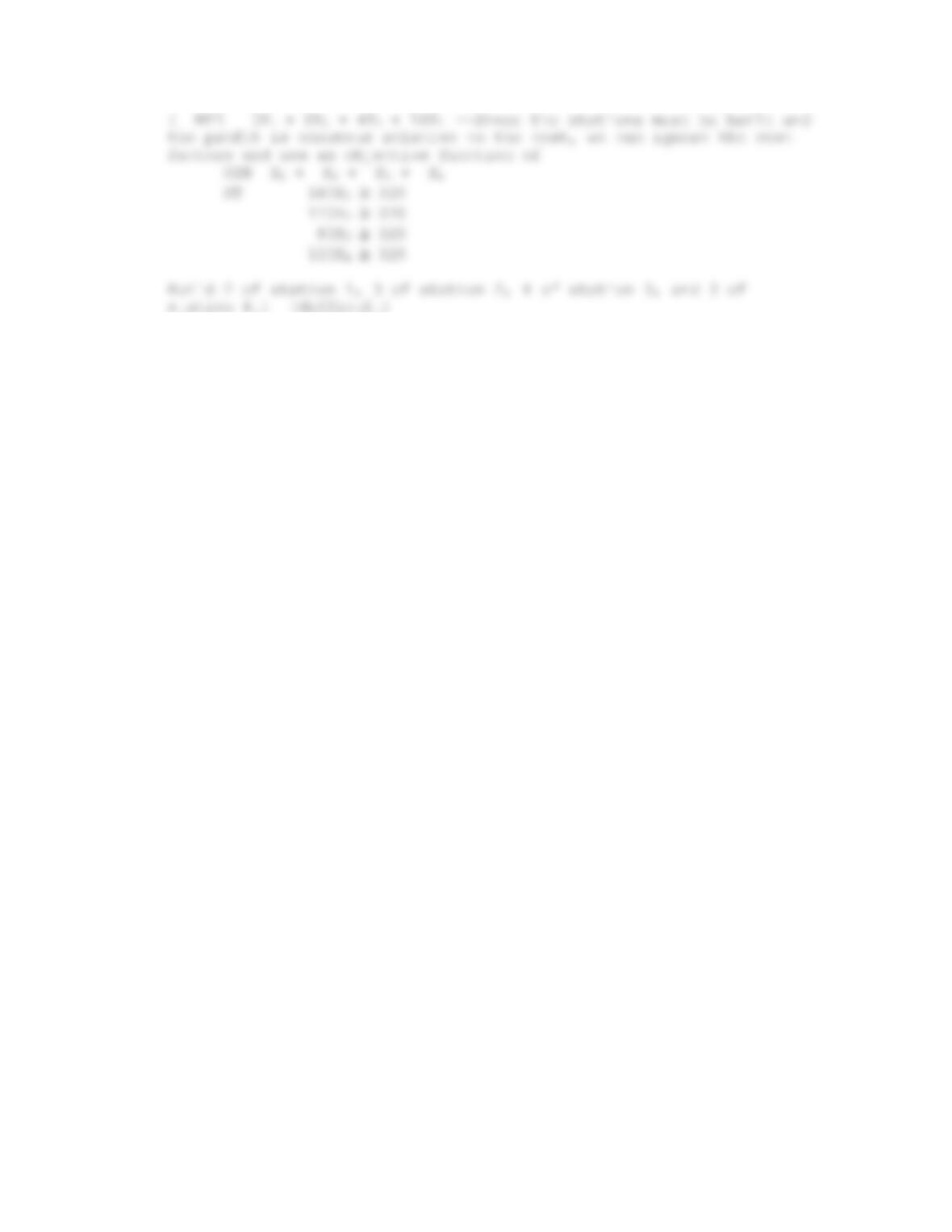
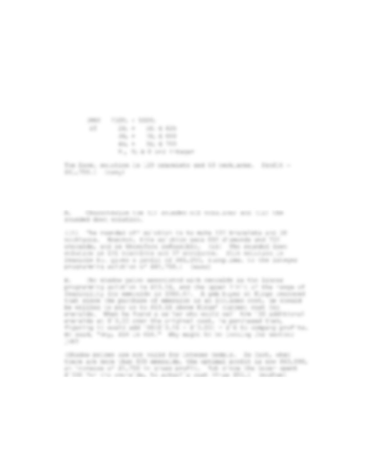
1. Kings Department Store has 625 rubies, 800 diamonds, and 700
emeralds from which they will make bracelets and necklaces that they
have advertised in their Christmas brochure. Each of the rubies is
approximately the same size and shape as the diamonds and the
emeralds. Kings will net a profit of $250 on each bracelet, which
is made with 2 rubies, 3 diamonds, and 4 emeralds, and $500 on each
necklace, which includes 5 rubies, 7 diamonds, and 3 emeralds. How
many of each should Kings make to maximize its profit?
2. The optimal linear programming solution to the Kings
Department Store problem in problem 1 is 131.58 bracelets and 57.89
necklaces.
3. Wisconsin State University is planning to advertise its new
degree program in Professional Business in several media—–television
commercials on the local cable station, advertisements in the local
community college newspaper, and manning a booth at the county fair.
Preliminary estimates are that each television spot will reach 1000
potential students, each newspaper ad will reach 100 potential
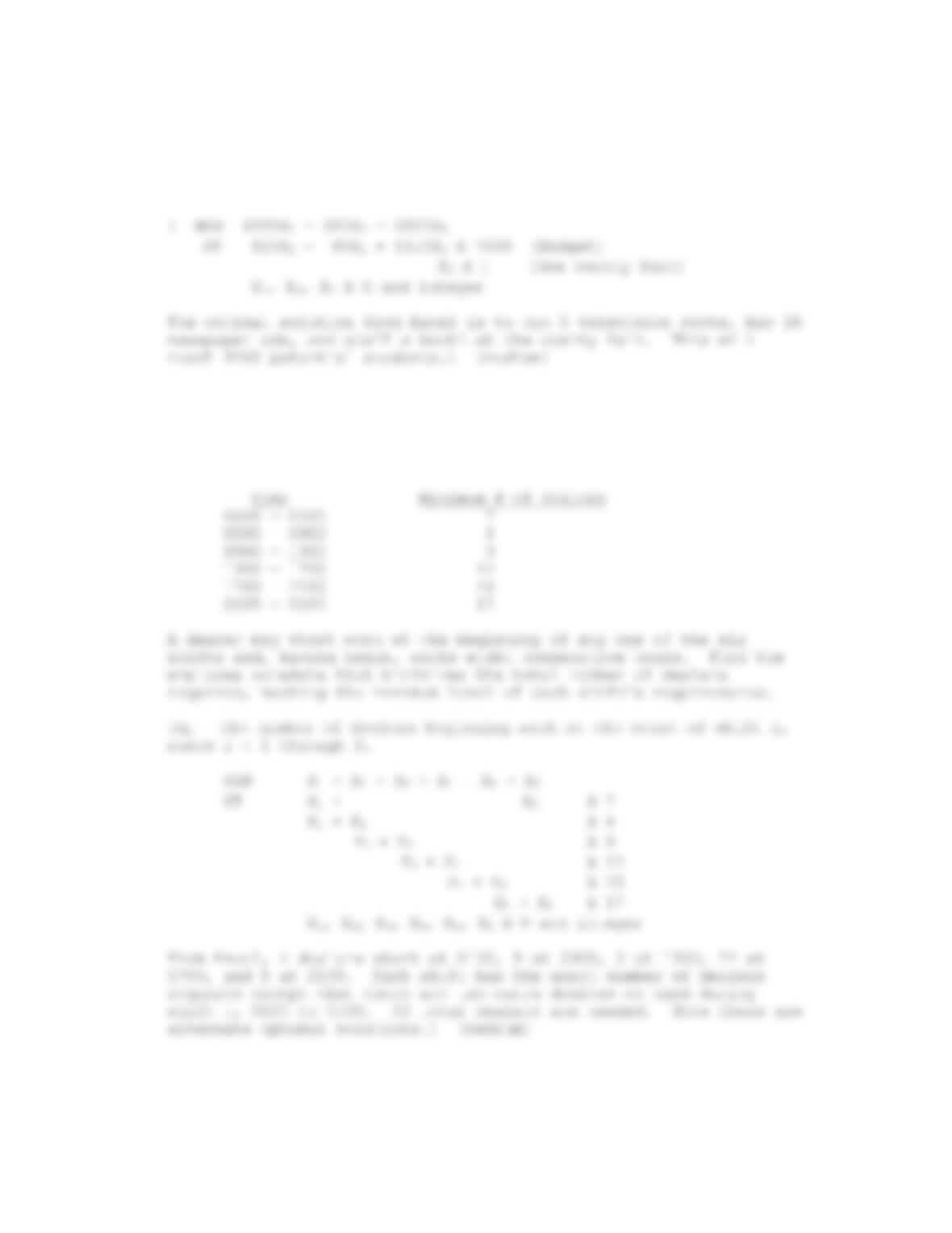
students, and each day at the county fair will reach 500 potential
students. There is a $7500 advertising budget, and the university
has negotiated a rate of $825 per ad on the cable station, $85 per
ad in the newspaper, and $1150 for a booth at the 3-day county fair.
What should be its advertising strategy?
4. Clancy’s Casino, in Muledeer, Nevada, is open 24 hours a day,
seven days a week. Along with all the other attractions and
diversion, Clancy’s operates a variety of gaming tables. Dealers at
these tables are interchangeable. The casino has the following
daily requirements for dealers:
5. Suppose in problem 4, Clancy’s Casino pays a wage differential
depending on the hours worked. In particular, between midnight and
0700, it pays dealers $16 per hour, between 0700 and 1900 $10 per
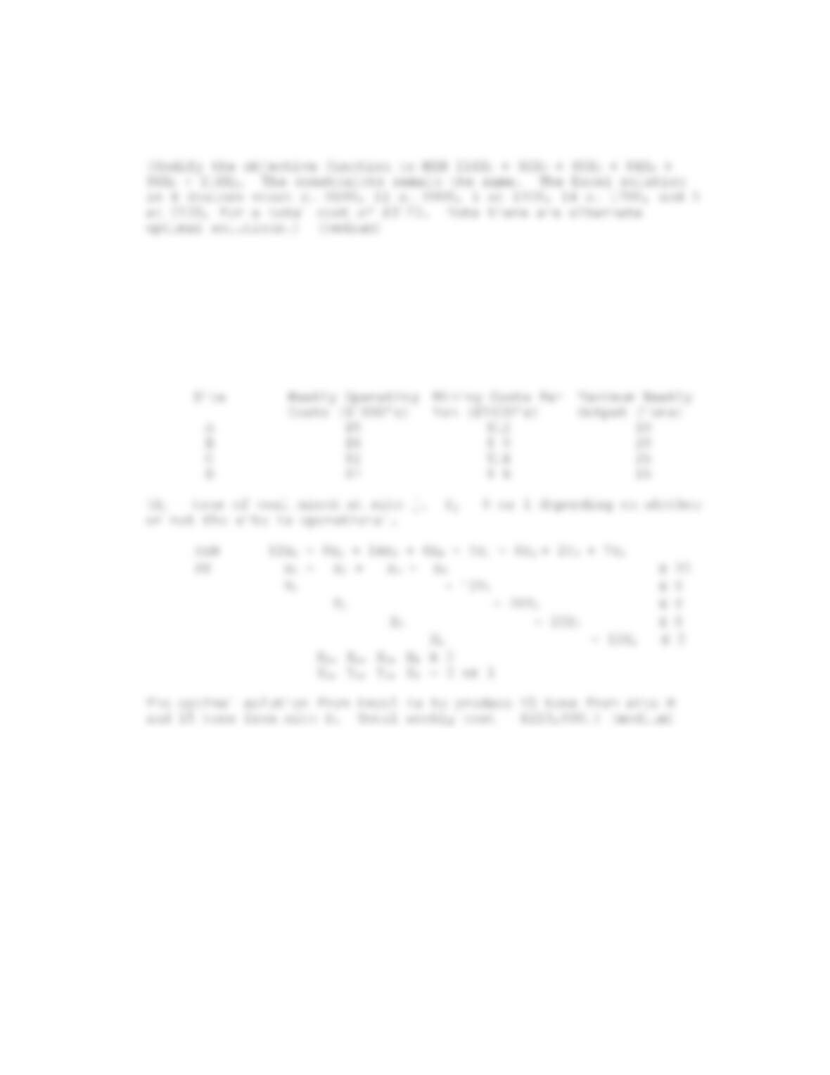
hour, and between 1900 and midnight $12 per hour. Modify your
formulation to problem 4, and determine the minimum cost shift
schedule for Clancy’s.
6. Appalachian Coal Company must mine a minimum of 30 tons of
coal weekly. It can mine at any of four sites. Relevant data
concerning fixed weekly operation costs of the sites, variable
mining costs per ton of coal, and estimated maximum weekly output of
coal at each site are given in the following table. Formulate a
mixed integer programming model and solve for the mining strategy
that will minimize total weekly costs.
7. Eastern Engineering Company is trying to decide which of 6
projects to perform during the next quarter. The net present value,
the estimated cost, and the number of engineers and staff personnel
required for each project are given in the following table.
Project
Net Present
Value
($1000’s)
Cost
($1000’s)
Engineers
Required
Staff
Required
1
100
35
5
2
2
145
65
8
3
3
200
95
11
2
4
250
180
4
2
5
500
250
16
7
6
695
475
19
11
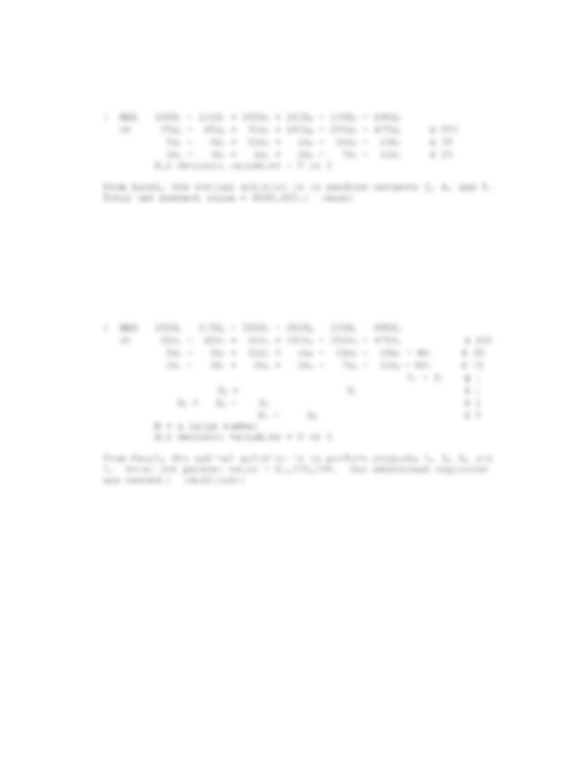
Eastern has a $550,000 budget and 30 engineers and 15 staff
available. Which projects should Eastern perform during the
quarter?
8. For the Eastern Engineering problem in question 7, suppose the
budget is increased to $600,000 and that the additional engineers or
additional staff (but not both) can be hired so that only one of the
engineer or staff limitations must hold (i.e. at least one of the
two constraints holds). Also, if project 2 is performed, project 5
will not be performed, at least two of projects 1, 2, and 3 should
be performed, and if project 3 is performed, project 4 should be
performed. Which projects should Eastern undertake under these
conditions?
9. Heavenly Casket Company is trying to choose sites for the
production of its “mail order” caskets. It is considering plants in
Chicago, Dallas, and Atlanta. Finished caskets will then be sent to
their two distribution sites in Trenton and Tacoma, which take
orders over the internet. Heavenly expects demand of 4000 caskets
per year in Trenton and 2500 in Tacoma. The table below gives
annual plant capacity, fixed yearly operating expenses, unit
production costs, and unit transportation costs between possible
plant locations and the distribution sites:
Site
Capacity
Fixed
Annual
Operating
Costs
Production
Cost Per
Unit
Shipping
to Trenton
Shipping
to Tacoma
Chicago
3500
$40,000
$200
75
50
Dallas
3200
$42,000
$160
95
70
Atlanta
3700
$45,000
$170
82
98
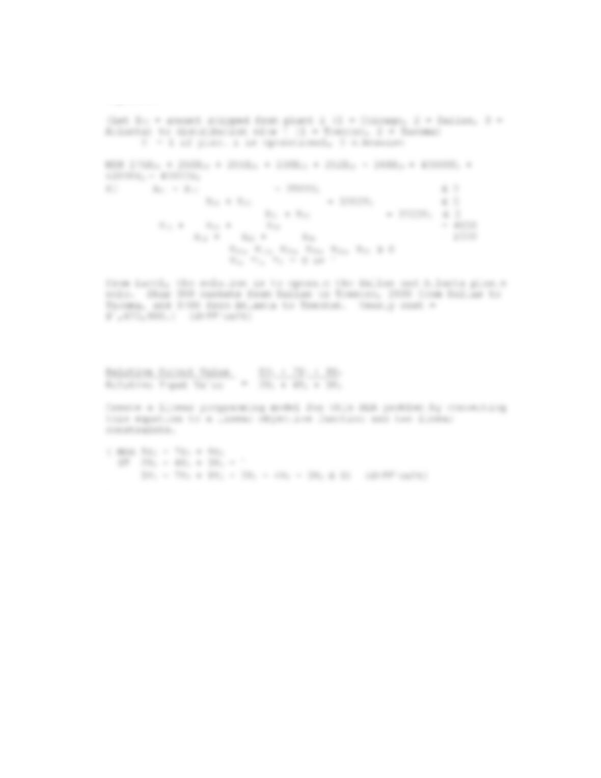
Which plants should be operational, and what should the production
quantities and shipping pattern be to minimize Heavenly’s annual
expenses?
10. The Data Envelopment Analysis model gives the following
equation:
11. An assembly line has 4 stations. All laborers are trained to
operate all stations. The union contract limits laborers to a 40
hour work week with no overtime. The company is contracted to
produce 320 units per week, with a profit of $1000 per unit. Each
unit must proceed through all 4 stations in order. However, there
is sufficient work in progress inventory to keep all stations busy
at all times. Station information is detailed in the following
table:
Station
Time Required Per
Unit in minutes
Cost to Build the
Station
1
15
$5000
2
20
$8000
3
30
$4000
4
20
$10,000
How many stations of each type does the assembly line require to
meet demand?