58. To measure the seasonal variation, we compute seasonal ____________________, which gauge the
degree to which the seasons differ from one another.
59. One application of seasonal indexes is to remove the seasonal variation in a time series. The process is
called ____________________, and the result is called a seasonally adjusted time series.
60. The easiest way of measuring the long-term trend is by ____________________ analysis, where time
is the independent variable.
61. A least squares ____________________ trend line is just a simple regression line with the years
recoded.
62. The easiest way of measuring the long-term trend is by regression analysis, where time is the
____________________ variable.
63. To create a seasonally adjusted time series, divide the time series by the seasonal
____________________.
ANS:
Holiday Hours
The total holiday hours (in 1000s) were recorded for 16 quarters in a large steel mill as shown below.
Year
Quarter
Overtime Hours
2011
1
32
2
15
3
21
4
28
2012
1
35
2
16
3
27
4
29
2013
1
36
2
21
3
25
4
37
2014
1
41
2
29
3
31
4
40
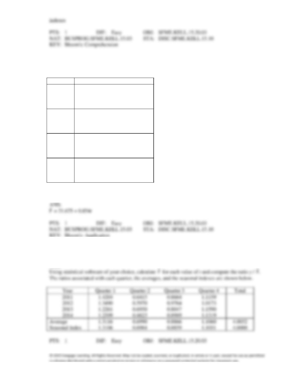
64. {Holiday Hours Narrative} Use the regression technique to calculate the linear trend line.
65. {Holiday Hours Narrative} Calculate the seasonal indexes based on the regression trend line in the
previous question.
ANS:
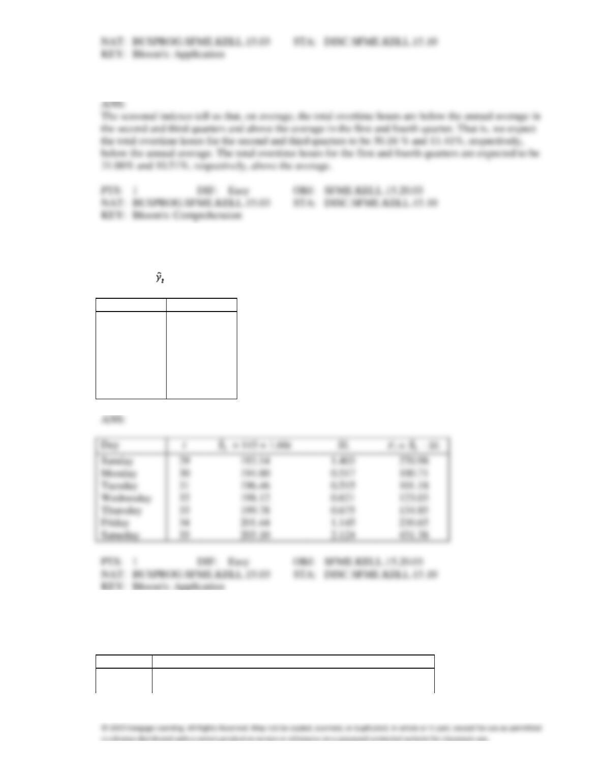
66. {Holiday Hours Narrative} What do the seasonal indexes tell us?
67. The trend line and seasonal indexes shown below were computed from four weeks of daily
observations. Forecast the seven values for the next week.
Trend Line: = 145 + 1.66t (t = 1,2,3,…28)
Day
SIt
Sunday
1.403
Monday
0.517
Tuesday
0.515
Wednesday
0.621
Thursday
0.675
Friday
1.145
Saturday
2.124
Sunday
1.403
Monday
0.517
Tuesday
0.515
Wednesday
0.621
Thursday
0.675
Friday
1.145
Saturday
2.124
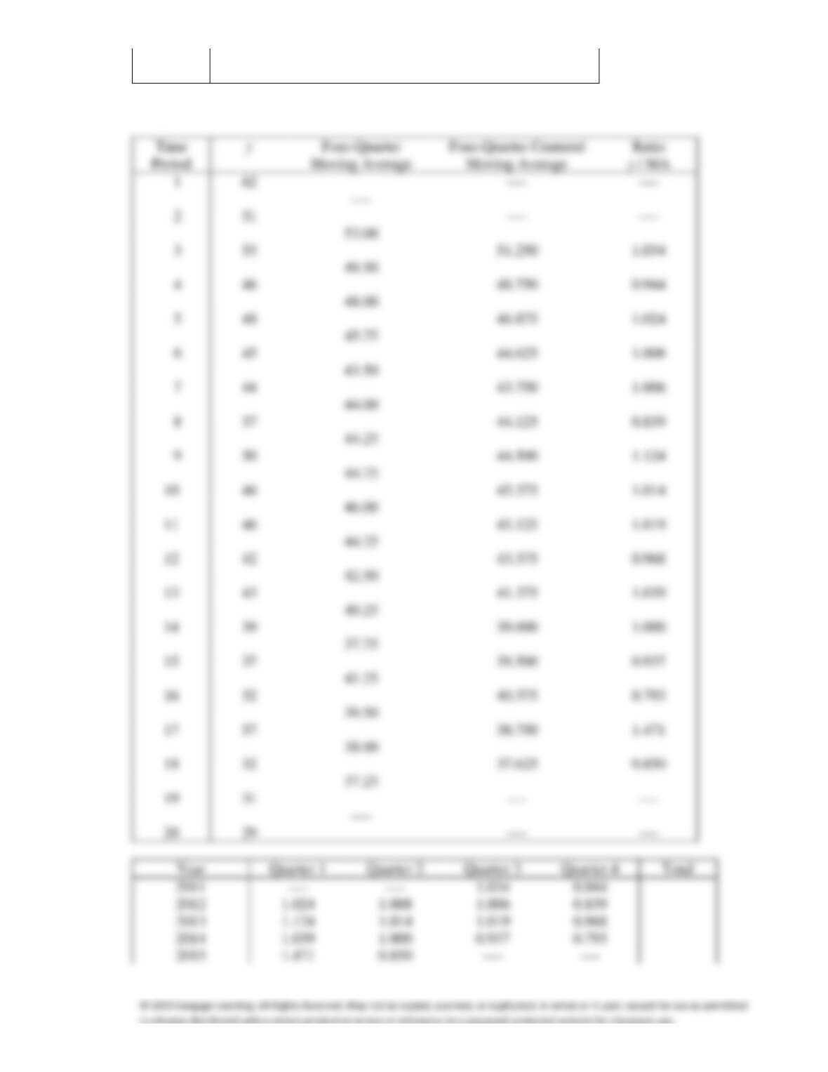
68. Given the following time series, compute the seasonal (quarterly) indexes, using the four-quarter
centered moving averages.
Year
Quarter
2011
2012
2013
2014
2015
1
62
48
50
43
57
2
51
45
46
39
32
3
53
44
46
37
31
4
46
37
42
32
29
ANS:
Moving Average
62
51
53
1.034
46
0.944
48
1.024
45
1.008
44
1.006
37
0.839
50
1.124
10
46
1.014
11
46
1.019
13
43
1.039
14
39
1.000
15
37
0.937
16
32
0.793
17
57
1.471
18
32
0.850
19
31
20
29
1.034
0.944
1.024
1.008
1.006
0.839
1.124
1.014
1.019
0.968
1.471
0.850
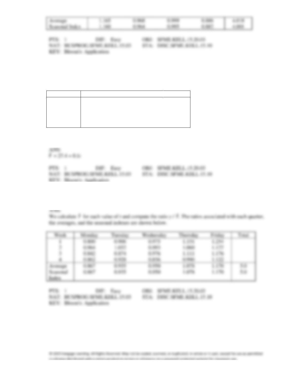
Average
1.165
0.968
0.999
0.886
Seasonal Index
1.160
0.964
0.995
0.882
Carpet Outlet
A carpet outlet has been keeping daily sales records over the past four weeks as shown below.
Week
Day
1
2
3
4
Monday
22
27
24
25
Tuesday
25
29
25
27
Wednesday
27
28
28
25
Thursday
32
30
32
29
Friday
35
32
34
33
69. {Carpet Outlet Narrative} Use the regression technique to calculate the linear trend line.
70. {Carpet Outlet Narrative} Calculate the daily indexes based on the regression trend line in the
previous question.
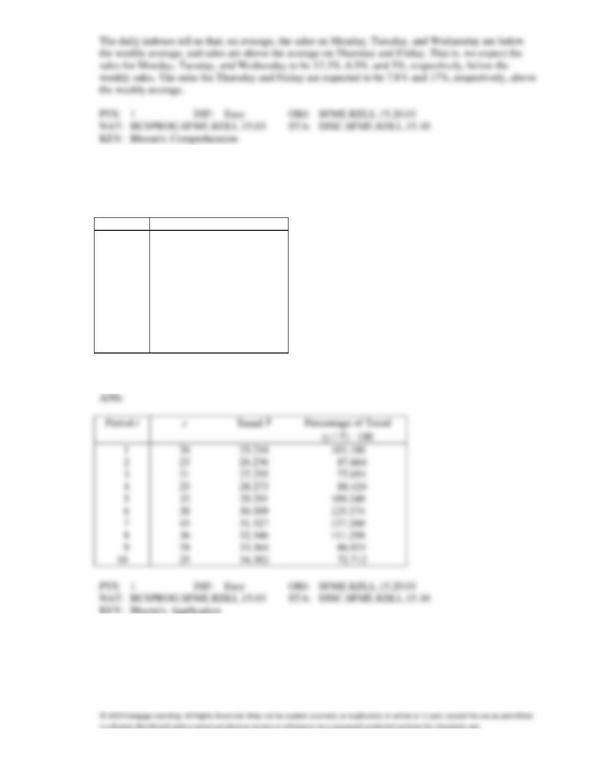
2
4
Average
Seasonal
Index
71. {Carpet Outlet Narrative} What do the daily indexes tell us?
ANS:
Microprocessors
Annual production (in millions) of computer microprocessors in a large electronics company was
recorded as shown below
Year
t
Production
2011
1
26
2012
2
23
2013
3
21
2014
4
25
2015
5
32
2016
6
38
2017
7
43
2018
8
36
2019
9
29
2020
10
25
72. {Microprocessors Narrative} Calculate the percentage of trend for each time period.
26
23
21
25
32
38
43
36
29
73. {Microprocessors Narrative} Plot the percentage of trend.
ANS:
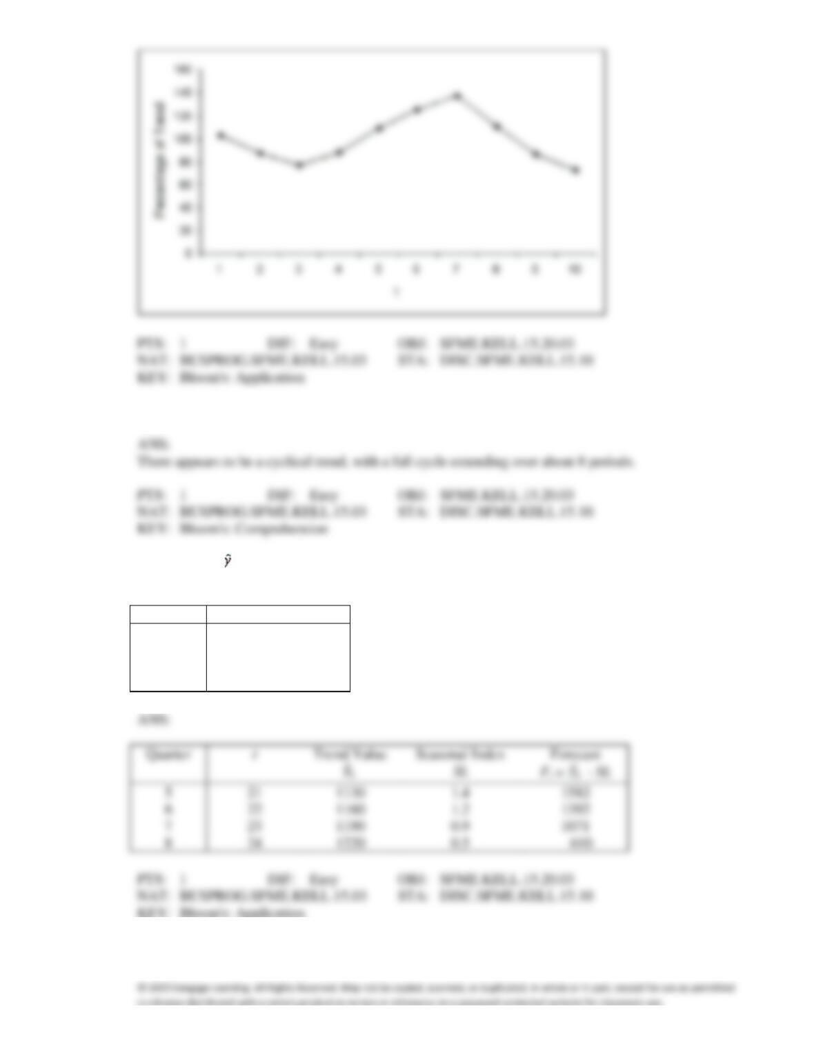
74. {Microprocessors Narrative} Describe the cyclical effect (if there is one).
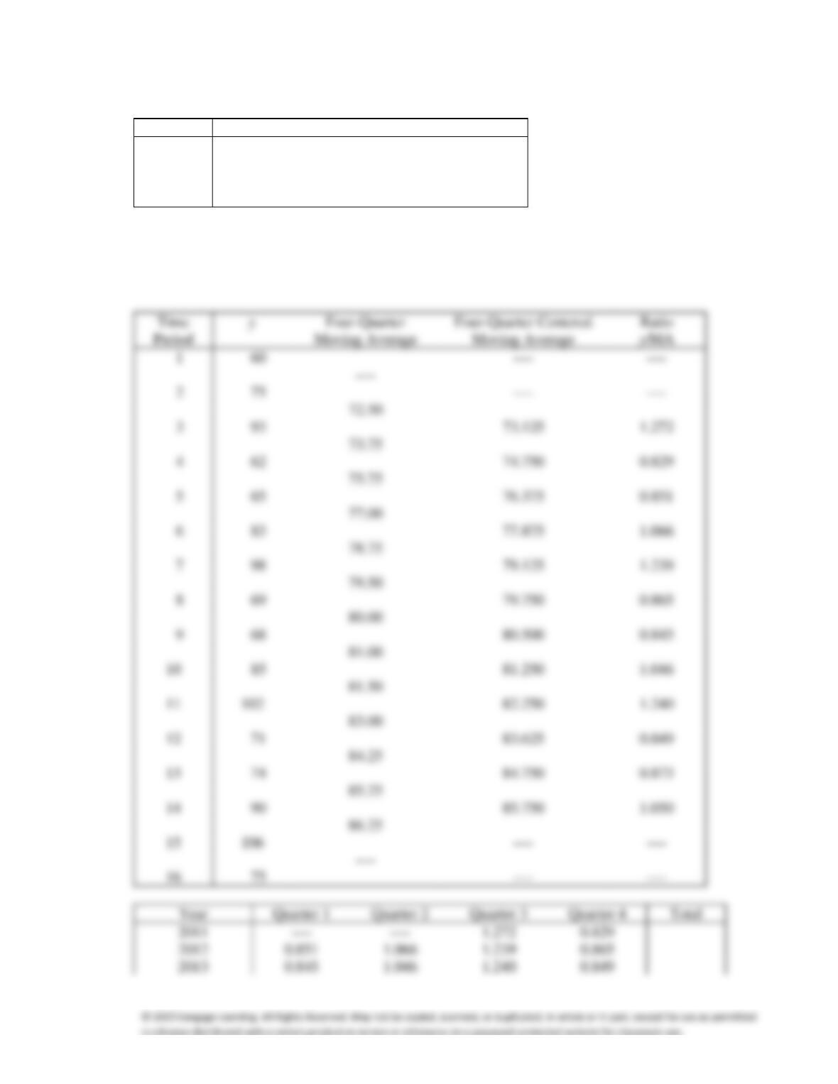
75. The trend line = 500 + 30t, (t = 1, 2, 3, …., 20), and the seasonal indexes shown in the table below
were computed from five years of quarterly sales data. Forecast the sales for the next four quarters.
Quarter
Seasonal Index
1
1.4
2
1.2
3
0.9
4
0.5
Quarter
5
6
7
8
76. The quarterly earnings of a large microcomputer company have been recorded for the years
2011-2014. These data (in millions of dollars) are shown in the accompanying table.
Year
Quarter
2011
2012
2013
2014
1
60
65
68
74
2
75
83
85
90
3
93
98
102
106
4
62
69
71
75
Use an appropriate moving average to measure the quarterly variation by computing the seasonal
(quarterly) indexes.
ANS:
Moving Average
60
—-
1.272
62
0.829
65
0.851
83
1.066
0.865
0.845
10
85
1.046
11
1.240
12
71
0.849
13
0.873
14
1.050
15
16
75
1.272
0.829
0.845
1.046
1.240
0.849
0.873
1.050
—-
—-
0.856
1.054
1.250
0.848
0.854
1.052
1.248
0.846
77. The trend line = 125 + 2t and seasonal indexes shown in the table below were computed from 10
years of quarterly data. Forecast the values for the next four quarters.
Quarter
SIt
1
0.6
2
1.3
3
1.6
4
0.5
ANS:
1
0.6
2
1.3
3
1.6
4
0.5
ebay Storefront Sales
The sales figures (in $1000s) have been recorded in an ebay storefront as shown in the following table.
Time Period
y
Time Period
y
1
35
9
46
2
32
10
43
3
29
11
48
4
26
12
41
5
28
13
34
6
32
14
29
7
38
15
25
8
43
16
23
78. {ebay Storefront Sales Narrative} Calculate the percentage of trend for each time period.
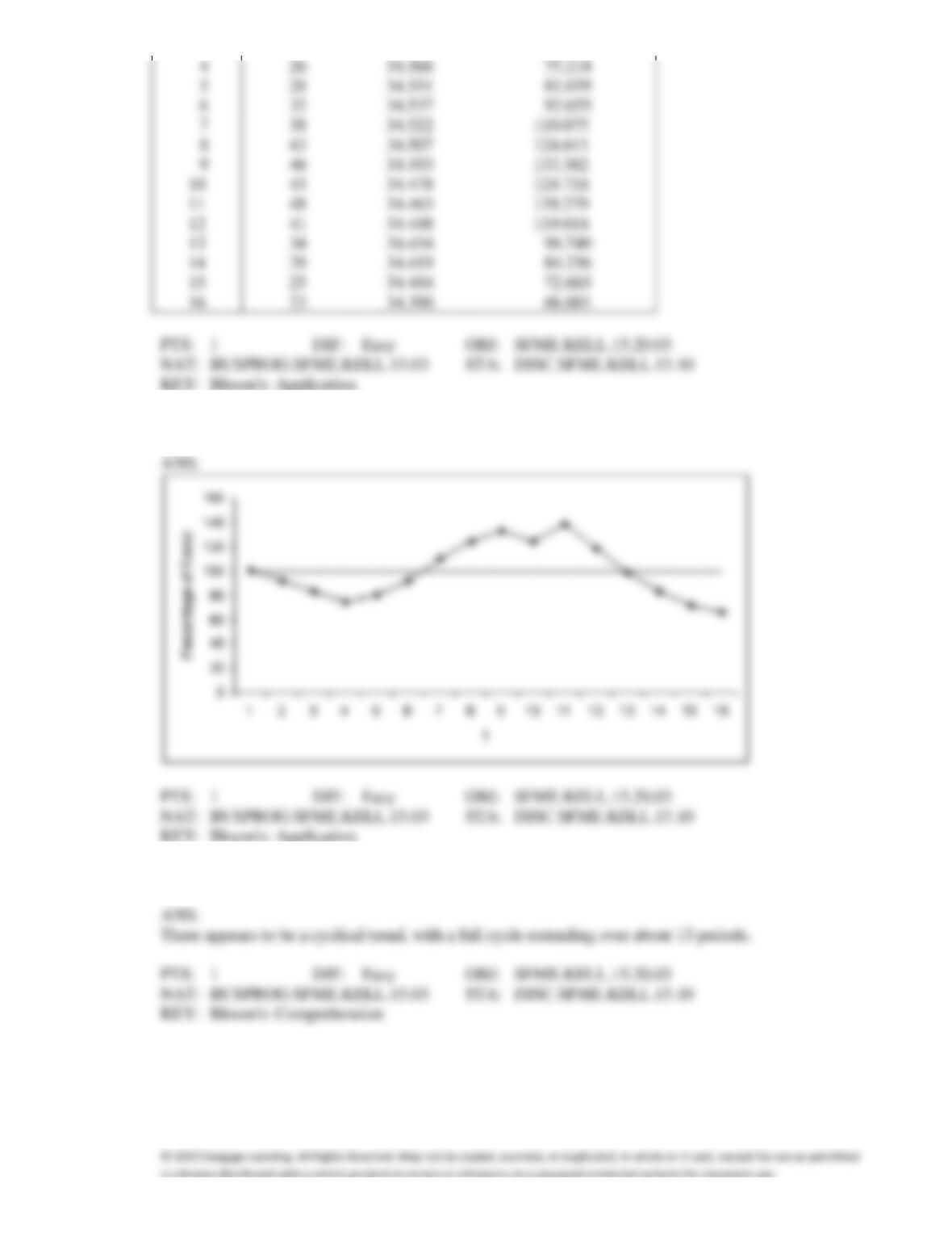
79. {ebay Storefront Sales Narrative} Plot the percentage of trend.
80. {ebay Storefront Sales Narrative} Describe the cyclical effect (if there is one).
Photo Equipment Store Earnings
The quarterly earnings of a chain of Photo Equipment stores have been recorded for the years
2011-2014. These data (in millions of dollars) are shown in the accompanying table.
Year
Quarter
2011
2012
2013
2014
1
65
70
73
79
2
80
88
90
95
3
98
103
107
111
4
67
74
76
80
81. {Photo Equipment Store Earnings Narrative} Develop a regression model, using indicator variables to
represent quarters.
82. {Photo Equipment Store Earnings Narrative} Forecast the quarterly earnings for the years 2015 and
2016.
83. Regression analysis was used to develop the following equation from 60 observations of quarterly
data: = 2500 − 3t − 3Q1 + 2Q2 + 5Q3, where
Forecast the next four quarters.
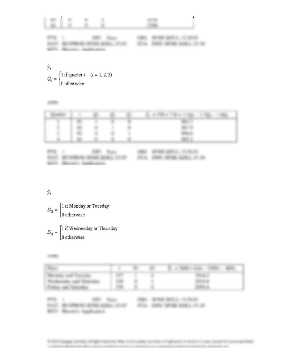
84. Regression analysis with t = 1 to 80 was used to develop the following forecast equation:
= 250 + 7.8t + 1.4Q1 − 1.7Q2 − 1.4Q3, where
Forecast the next four values.
85. A local newspaper that appears six days per week wanted to forecast two-day revenues from its
business services classified ads section. The revenues (in $1,000s) were recorded for the past 52
weeks. From these data, the following regression equation was computed:
= 2000 + 0.6t − 150D1 − 40D2 (t = 1, 2, 3, …, 156)
where
and
Forecast the two-day revenues for the next week.
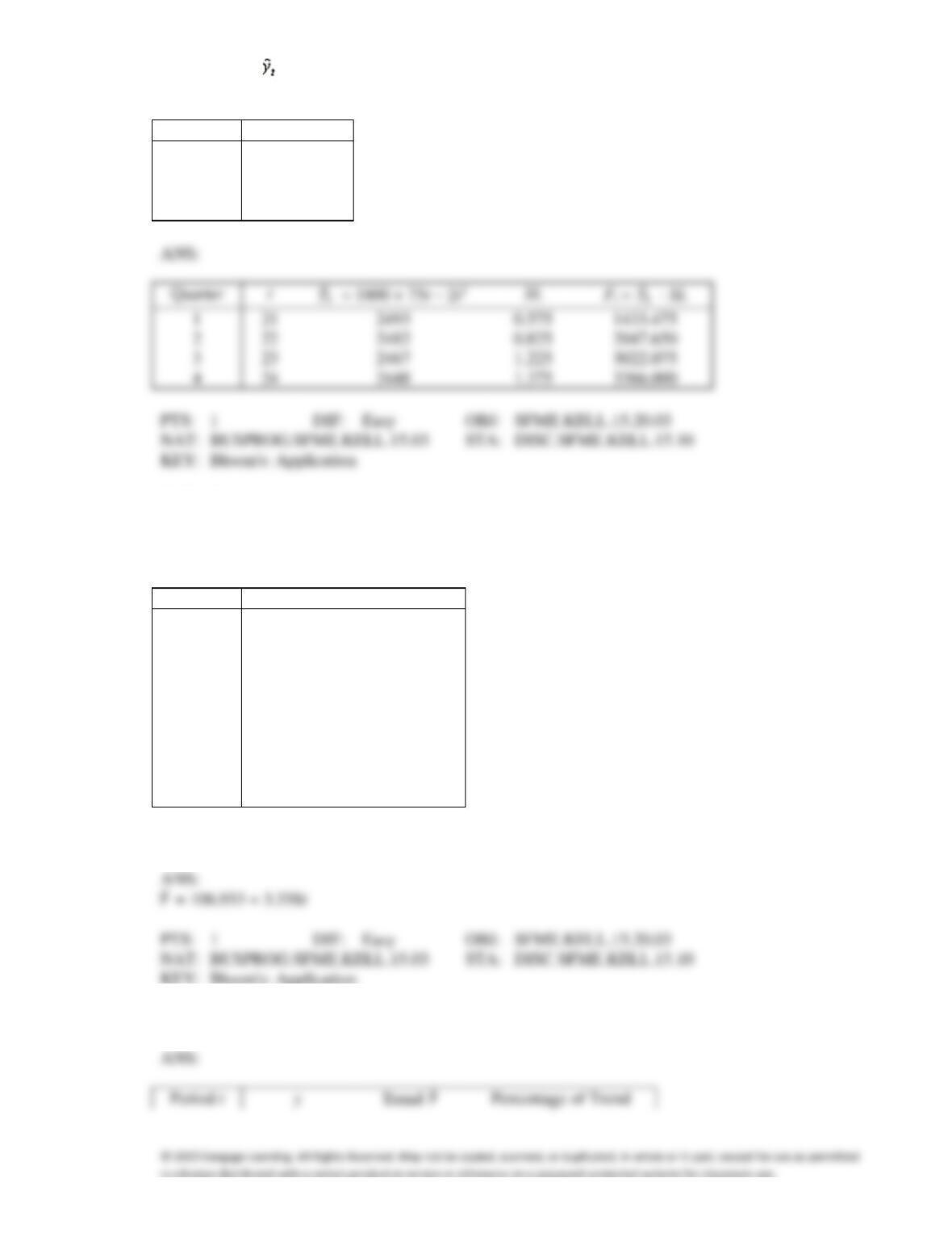
86. The trend line = 1800 + 75t − 2t2 and seasonal indexes shown in the table below were computed
from five years of quarterly observations. Forecast the four quarterly values for next year.
Quarter
SIt
1
0.575
2
0.825
3
1.225
4
1.375
1
21
2
22
3
4
24
Coffee Imports
The coffee imports (in millions of dollars) from a Latin American country for 10 years are shown
below.
Year
t
Exports
2011
1
96
2012
2
110
2013
3
125
2014
4
141
2015
5
132
2016
6
126
2017
7
118
2018
8
125
2019
9
133
2020
10
148
87. {Coffee Imports Narrative} Use the regression technique to calculate the linear trend line.
88. {Coffee Imports Narrative} Calculate the percentage of trend.
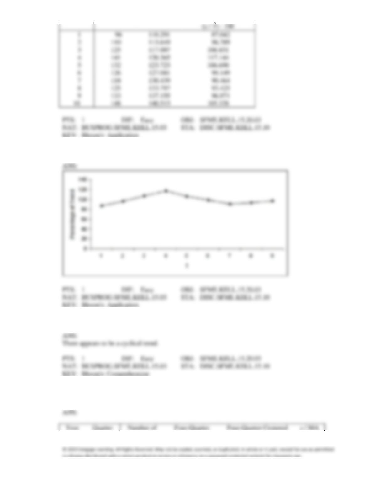
89. {Coffee Imports Narrative} Plot the percentage of trend.
90. {Agricultural Exports Narrative} Describe the cyclical effect (if there is one).
91. {The Pyramids of Giza Narrative} Calculate the four-quarter centered moving averages and use it to
calculate the seasonal (quarterly) indexes.