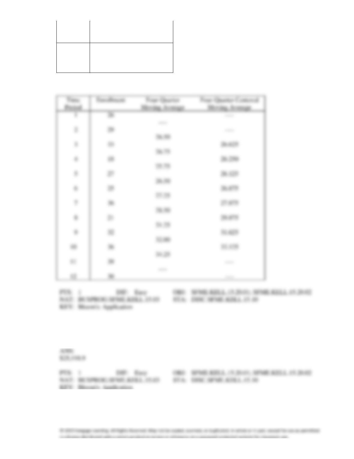
2
25
3
36
4
21
2013
1
32
2
36
3
39
4
30
ANS:
26
29
33
18
27
25
36
21
32
36
39
30
6. The manager of a lingerie store believed that her store profits were following an exponential trend. She
used statistical software to obtain the following prediction equation of profits: log10(Profits) = 2 +
0.4X. The data she used were from 2011 through 2016, coded 0 to 5. Find the forecast of 2017 profits.
7. Use exponential smoothing, with w = 0.4, to forecast the next value of the time series that follows.
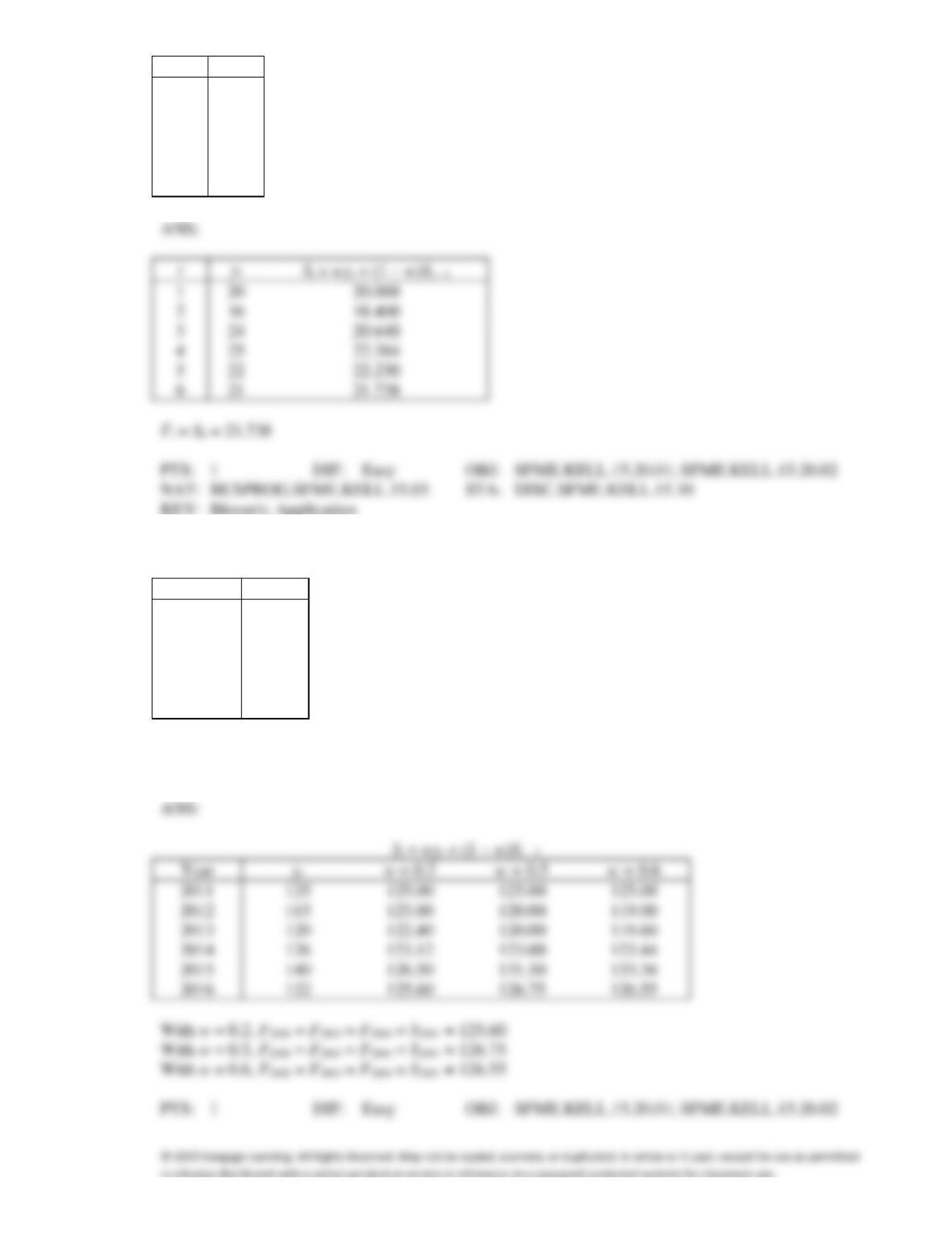
t
yt
1
20
2
16
3
24
4
25
5
22
6
21
1
20
2
16
3
24
4
25
5
22
6
21
8. A time series for the years 2011-2016 is shown below.
Year
yt
2011
125
2012
115
2013
120
2014
126
2015
140
2016
122
Develop forecasts for the years 2002-2004, with the following smoothing constant values: w = 0.2, w =
0.5, and w = 0.6.
Year
2011
2012
2013
2014
2015
2016
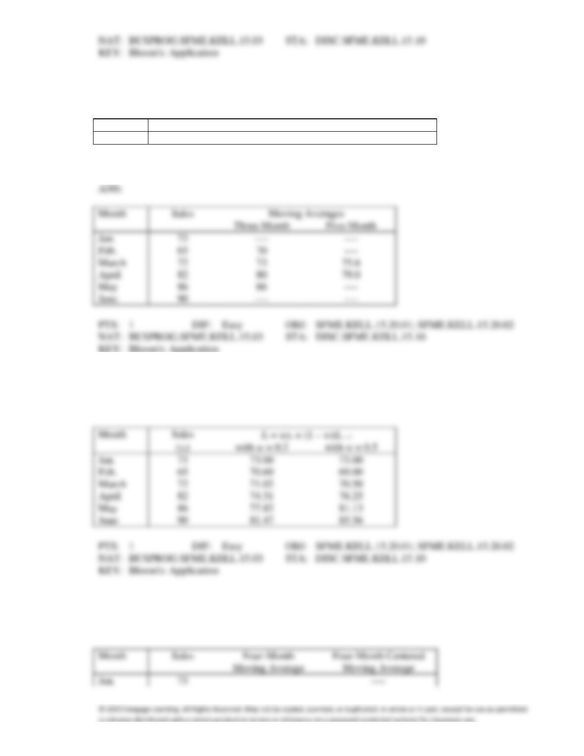
Mattress Sales
Monthly mattress sales (in $1,000s) of a mattress store are shown below.
Month
Jan.
Feb.
March
April
May
June
Sales
73
65
72
82
86
90
9. {Monthly Mattress Sales Narrative} Compute the three-month and five-month moving averages.
Month
Jan.
Feb.
March
April
June
10. {Monthly Mattress Sales Narrative} Compute the exponentially smoothed sales with w = 0.3 and w =
0.5.
ANS:
with w = 0.3
with w = 0.5
Jan.
Feb.
March
April
June
11. {Monthly Mattress Sales Narrative} Calculate the four-month moving average, and four-month
centered moving average.
ANS:
Jan.
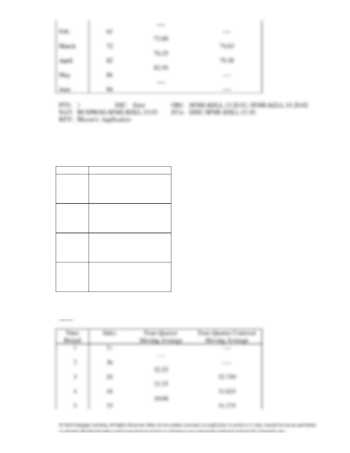
65
72
82
86
90
Quarterly Sales
The quarterly sales (in millions of dollars) of a Motorcycle Dealership were recorded for the years
2011-2014. They are listed below.
Year
Quarter
Sales
2011
1
21
2
36
3
28
4
44
2012
1
25
2
23
3
39
4
36
2013
1
30
2
41
3
47
4
55
2014
1
34
2
29
3
32
4
48
12. {Quarterly Sales Narrative} Calculate the four-quarter centered moving averages.
21
36
28
44
25
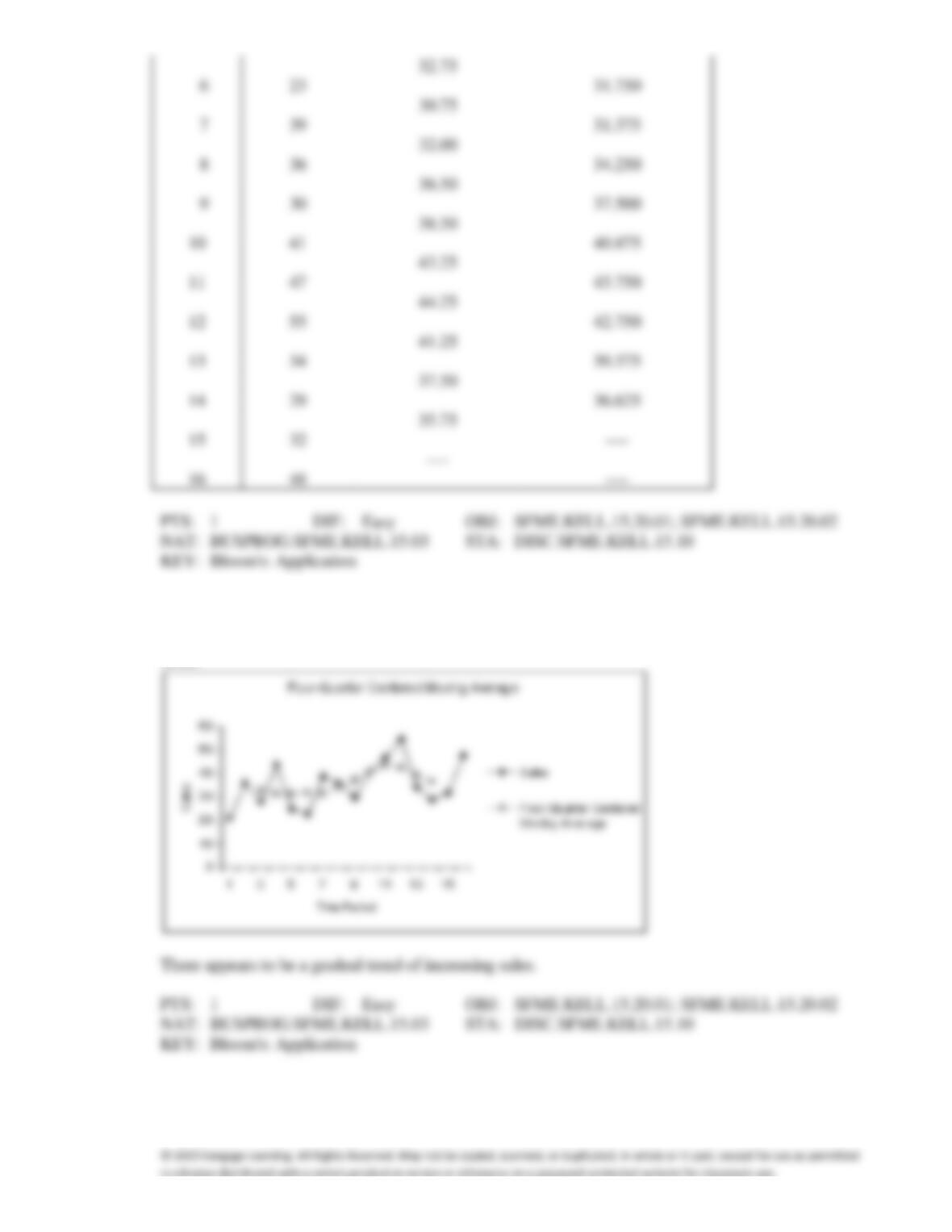
13. {Quarterly Sales Narrative} Graph the time series and the moving averages. What can you conclude
from your time-series smoothing?
ANS:
The Pyramids of Giza
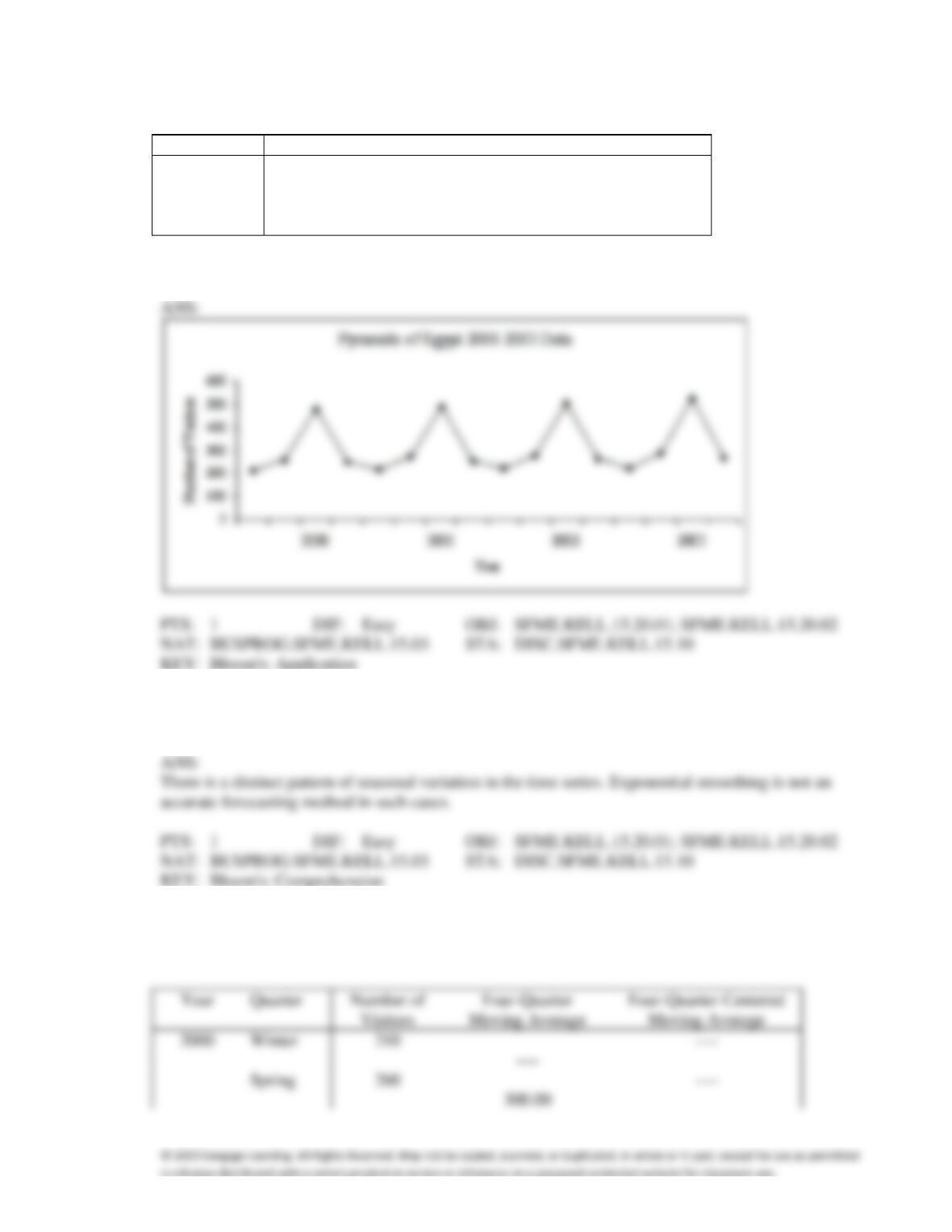
The Pyramids of Giza is one of the most visited monuments in Egypt. The number of visitors per
quarter has been recorded (in thousands) as shown in the accompanying table:
Year
Quarter
2000
2001
2002
2003
Winter
210
215
218
220
Spring
260
275
282
290
Summer
480
490
505
525
Fall
250
255
265
270
14. {The Pyramids of Giza Narrative} Plot the time series.
15. {The Pyramids of Giza Narrative} Discuss why exponential smoothing is not recommended as a
forecasting method in this case.
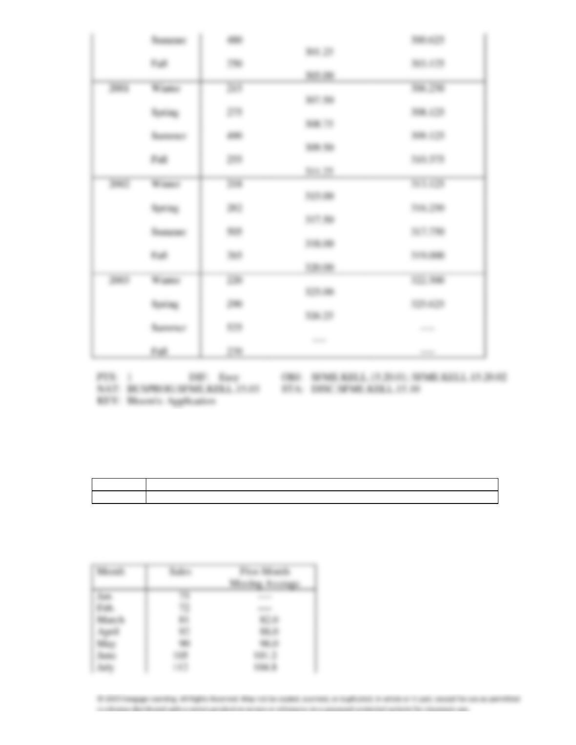
16. {The Pyramids of Giza Narrative} Calculate the four-quarter centered moving averages.
ANS:
Quarter
Four-Quarter
Winter
210
Spring
260
Summer
Fall
Winter
Spring
Summer
Fall
Winter
Spring
Fall
Winter
Spring
Summer
Fall
Biodiesel Sales
Biodiesel (a vegetable oil or animal fat based diesel fuel) sales in Nebraska have been recorded over
the past 10 months as shown below.
Month
Jan.
Feb.
March
April
May
June
July
Aug.
Sept.
Oct.
Sales
75
72
81
92
90
105
112
107
110
93
17. {Biodiesel Sales Narrative} Compute the five-month moving average.
ANS:
Month
Jan.
Feb.
March
April
June
July
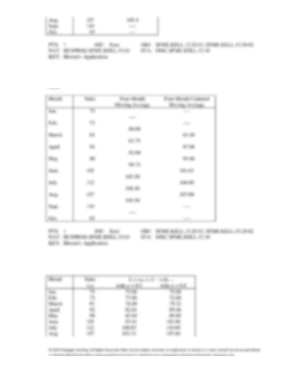
18. {Biodiesel Sales Narrative} Calculate the four-month moving average, and four-month centered
moving average.
ANS:
19. {Biodiesel Sales Narrative} Compute the exponentially smoothed sales with w = 0.4 and w = 0.8.
ANS:
Sept.
110
Oct.
93
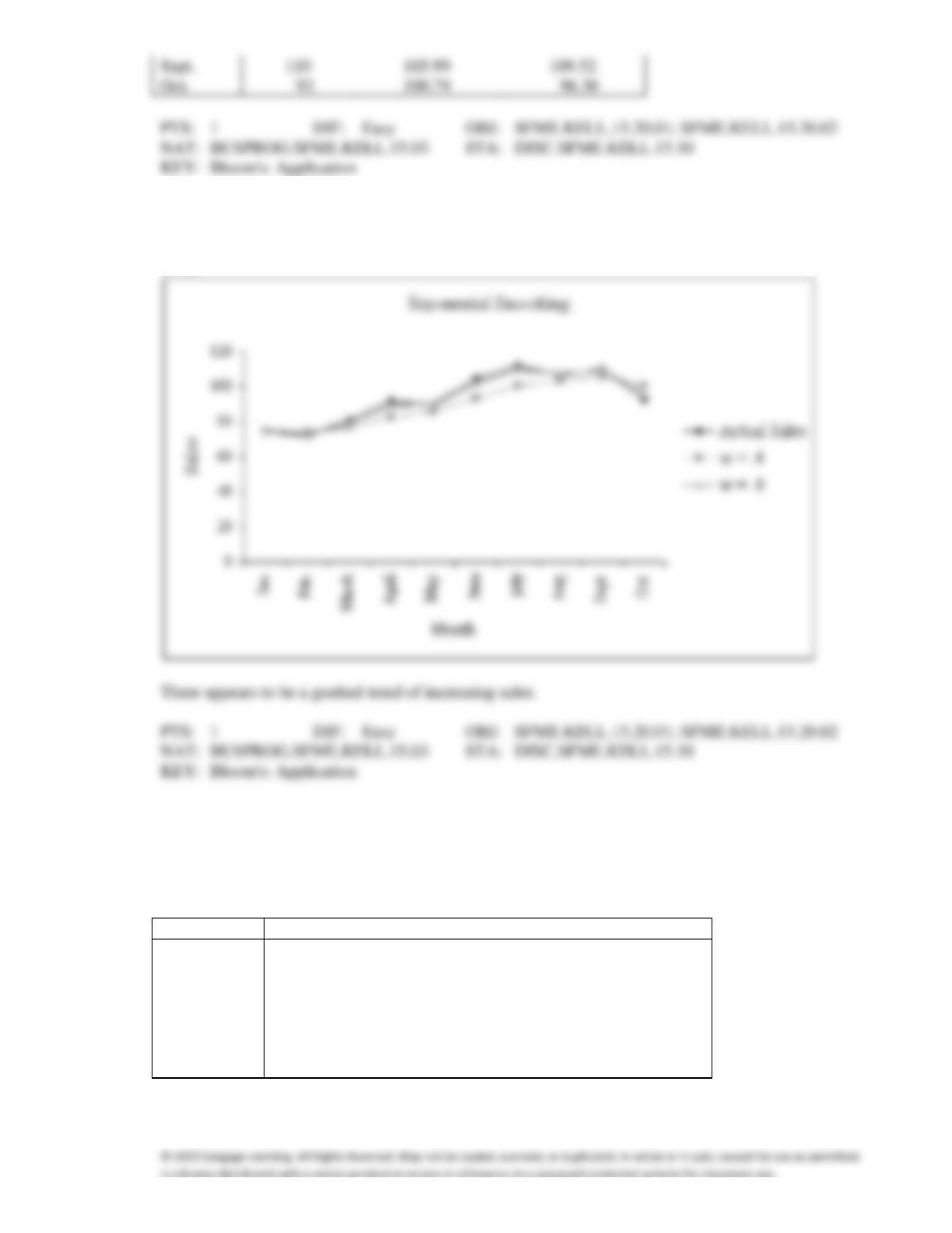
20. {Biodiesel Sales Narrative} Draw the time series and the two sets of exponentially smoothed values.
Does there appear to be a trend component in the time series?
ANS:
Daily Hoagie Sales
The table below shows the number of hoagies sold daily during a four-week period at Hoagie Haven in
Sutton, West Virginia.
Week
Day
1
2
3
4
Sunday
253
234
248
232
Monday
98
93
99
104
Tuesday
106
88
87
115
Wednesday
119
134
113
102
Thursday
138
123
130
118
Friday
201
215
218
205
Saturday
327
399
415
390
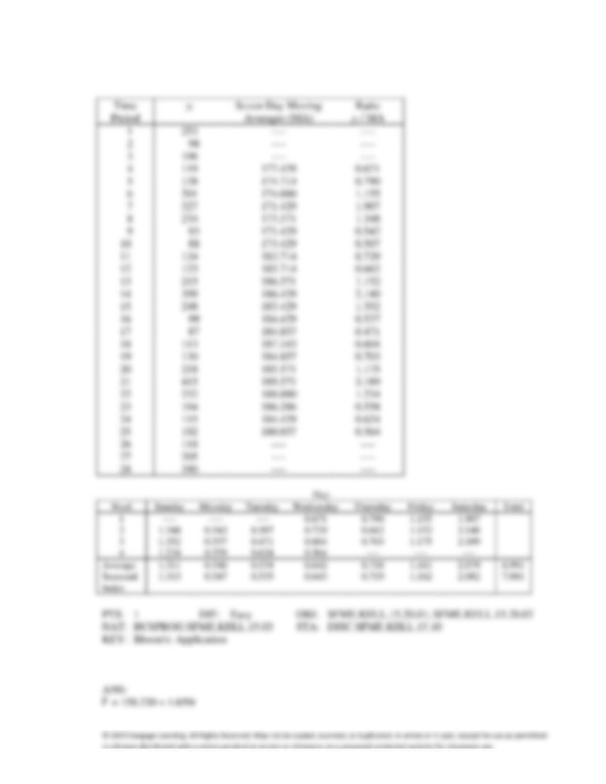
21. {Daily Hoagie Sales Narrative} Calculate the seasonal (daily) indexes, using a seven-day moving
average.
ANS:
22. {Daily Hoagie Sales Narrative} Use regression analysis to find the linear trend line.
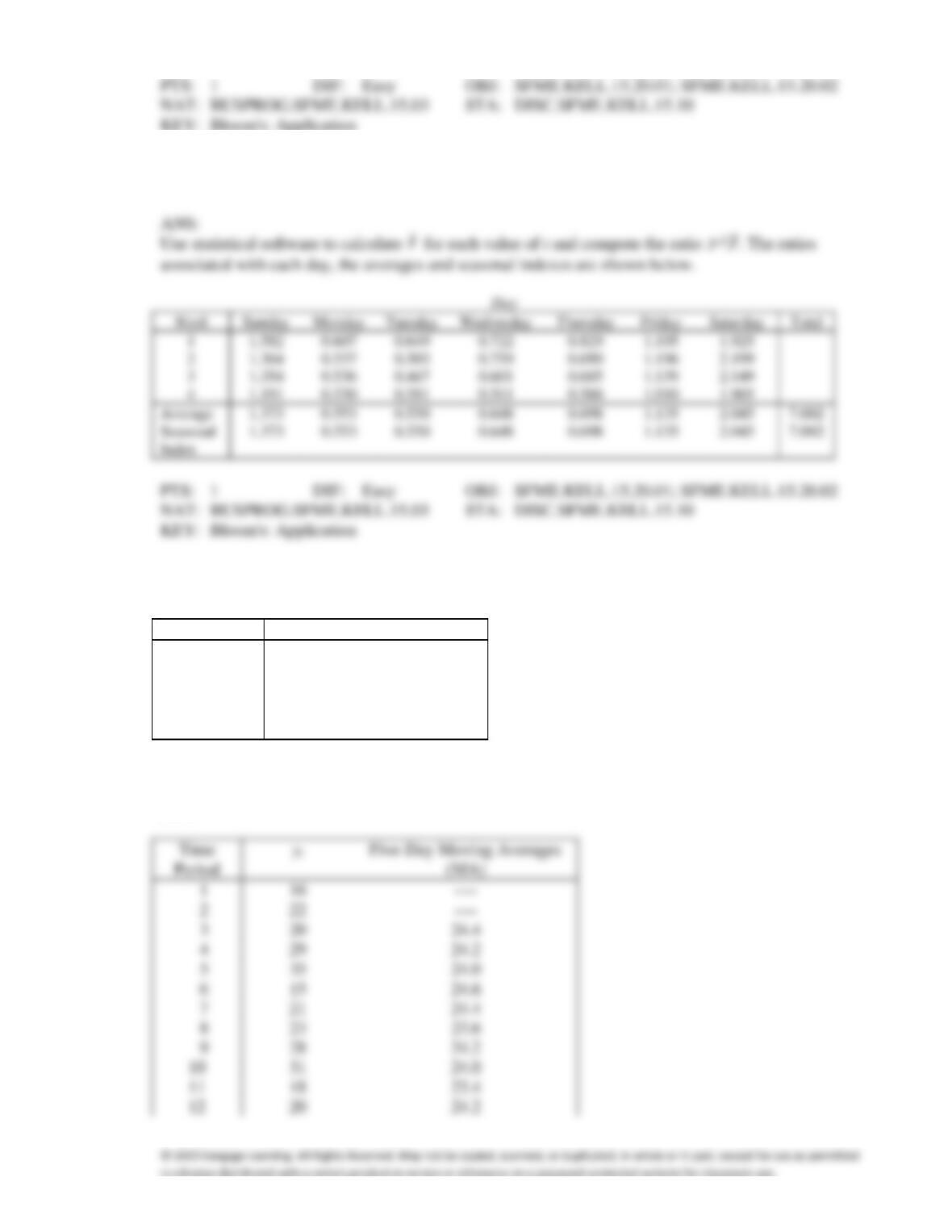
23. {Daily Hoagie Sales Narrative} Calculate the seasonal (daily) indexes, using the trend line developed
in the previous question.
24. A time series is shown in the table below:
Week
Day
1
2
3
4
Monday
16
15
18
21
Tuesday
22
21
20
25
Wednesday
20
23
20
24
Thursday
29
28
32
28
Friday
35
31
29
36
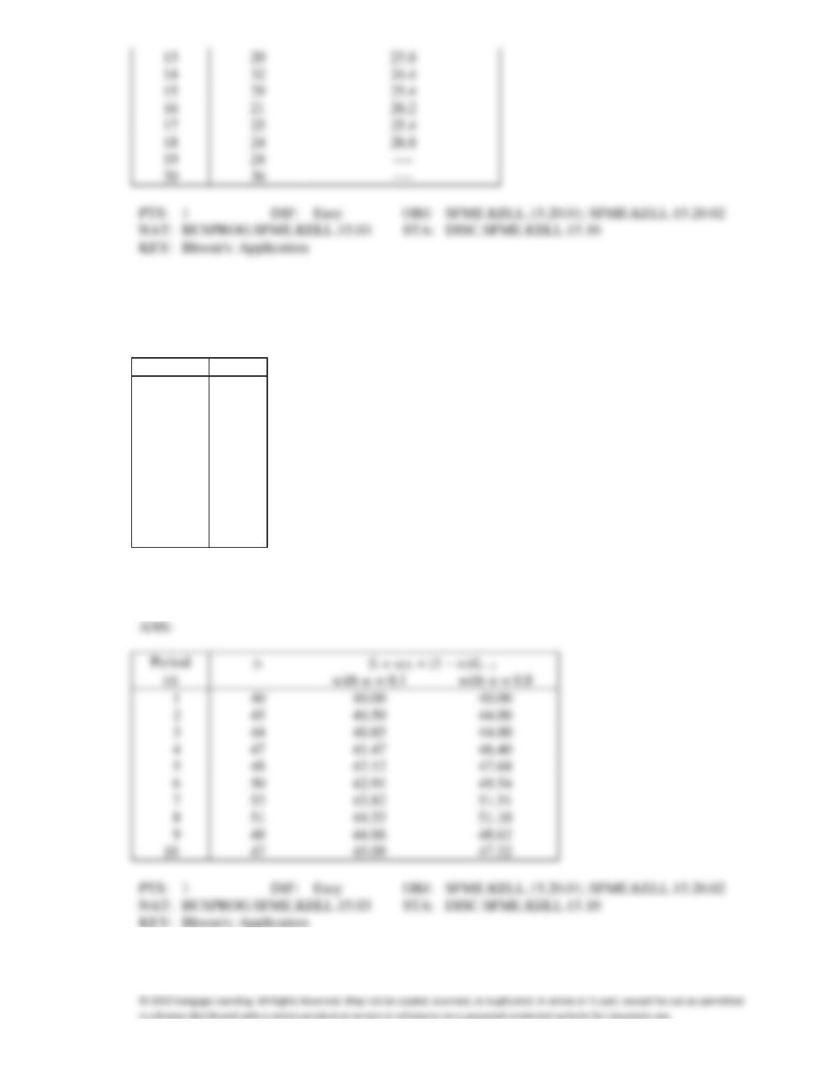
Compute the five-day moving averages to remove the seasonal and random variation.
ANS:
14
16
19
Motor Oil Sales
As part of an effort to forecast future sales, the monthly motor oil sales (in thousands of gallons) for
the past 10 months are recorded. These data are shown below.
Period t
yt
1
40
2
45
3
44
4
47
5
48
6
50
7
52
8
51
9
48
10
47
25. {Motor Oil Sales Narrative} Apply exponential smoothing with w = 0.1 and w = 0.8 to help detect the
components of the time series.
1
2
3
4
5
7
8
9
10
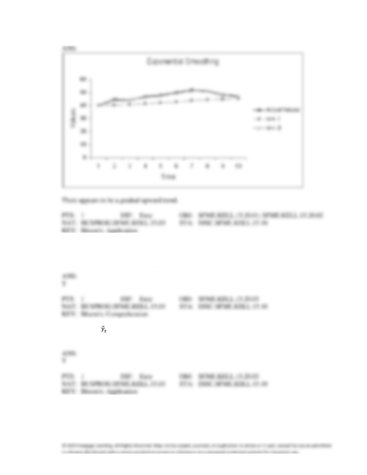
26. {Motor Oil Sales Narrative} Draw the time series and the two sets of exponentially smoothed values.
Does there appear to be a trend component in the time series?
27. In determining weekly seasonal indexes for natural gas consumption, the sum of the 52 means for gas
consumption as a percentage of the moving average is 5195. To get the seasonal indexes, each
monthly mean is to be multiplied by (5200 / 5195).
28. The trend line = 0.75 + 0.005t was calculated from quarterly data for 2000-2004, where t = 1 for
the first quarter of 2000. The trend value for the second quarter of the year 2005 is 0.86.
29. In determining monthly seasonal indexes for natural gas consumption, the sum of the 12 means for gas
consumption as a percentage of the moving average is 1195. To get the seasonal indexes, each
monthly mean is to be multiplied by (1195 / 1200).
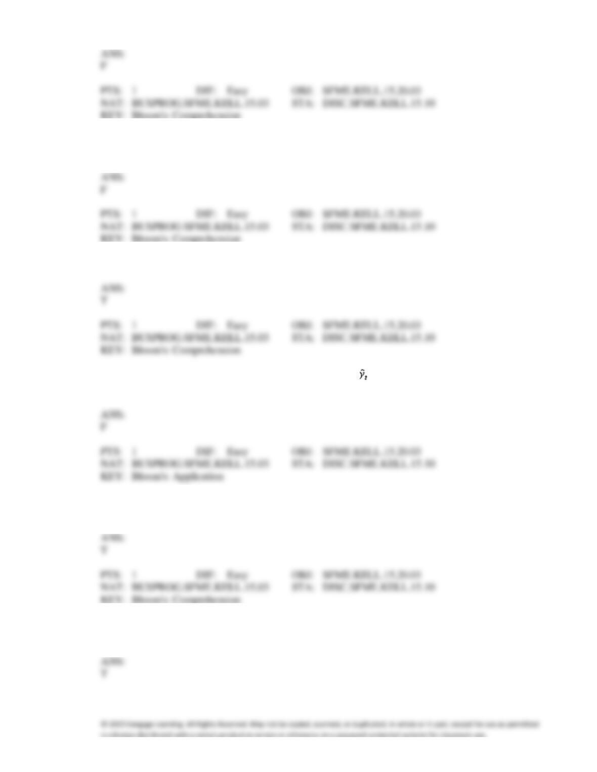
30. If summer 2011 sales were $16,800 and the summer seasonal index was 1.20, then the deseasonalized
2011 summer sales value was $20,160.
31. Seasonal variations will not be present in a deseasonalized time series.
32. The results of a quadratic model fit to time series data were = 8.5 − 0.25t + 2.5t2, where t = 1 for
1998. The forecasted value for 2005 is 129.25.
33. To measure the seasonal variation, we compute seasonal indexes, which gauge the degree to which the
seasons differ from one another.
34. One application of seasonal indexes is to remove the seasonal variation in a time series. The process is
called deseasonalizing, and the result is called a seasonally adjusted time series.
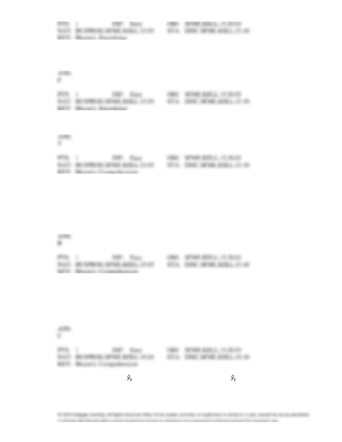
35. The easiest way of measuring the long-term trend is by regression analysis, where time is the
dependent variable.
36. A least squares linear trend line is just a simple regression line with the years recoded.
37. In determining monthly seasonal indexes, the first step is to construct a centered moving average with
a period of
a.
24 months
b.
12 months
c.
6 months
d.
3 months
38. Which of the following will not be present in a deseasonalized time series?
a.
Trend effects
b.
Cyclical variation
c.
Seasonal variation
d.
Random variation
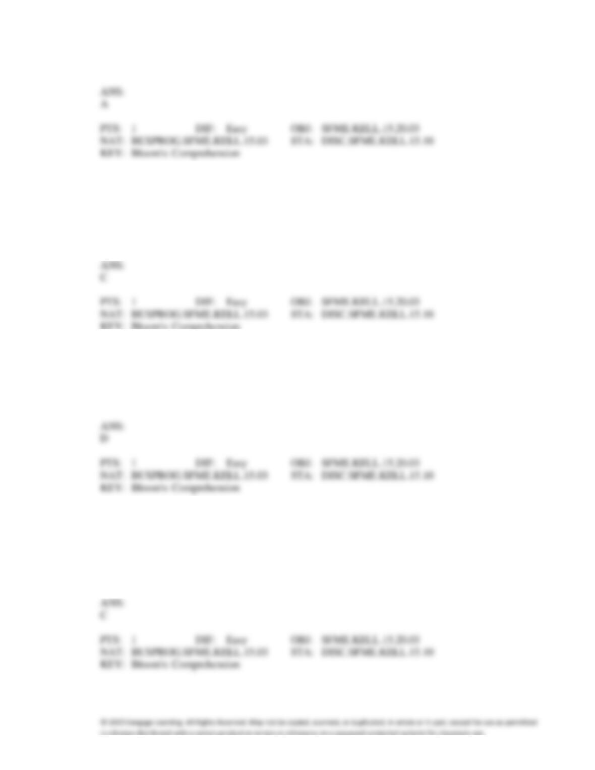
39. The term b1 in the equation = b0 + b1t + b2Q1 + b3Q2 +b4Q3, where represents the predicted
value of y at time t, is:
a.
time trend
b.
seasonal trend
c.
an indicator variable
d.
a value between 0 and 4
40. The level of construction employment in West Virginia is lowest during the winter. A model designed
to forecast construction employment in Charleston should use:
a.
a time trend
b.
a moving average
c.
seasonal indicator variable
d.
an autoregressive model
41. Which of the following will be reflected by deseasonalized time series?
a.
Trend effects
b.
Cyclical effects
c.
Random variation
d.
All of these choices are true.
42. Which of the following equations deseasonalize a time series, where T, C, S, and R are respectively the
trend, cyclical, seasonal, and random variation components of the time series?
a.
(T C S R) / T = C S R
b.
(T C S R) / C = T S R
c.
(T C S R) / S = T C R
d.
(T C S R) / R = T C S
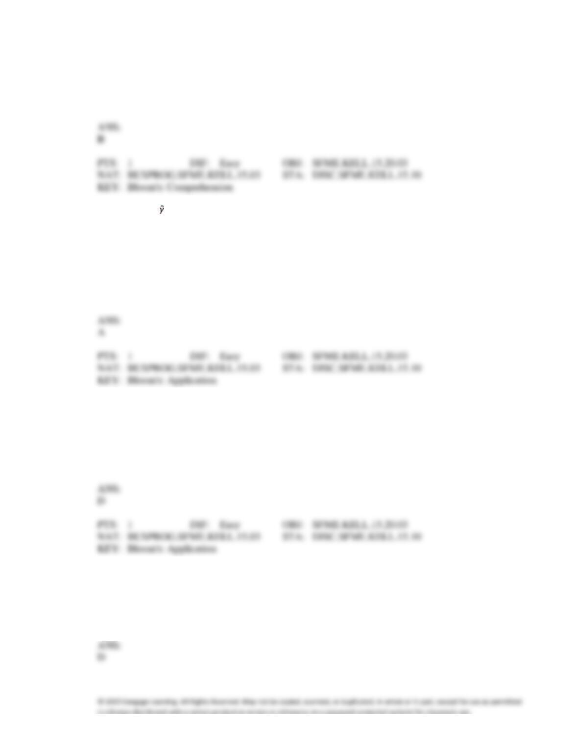
43. The linear model for long-term trend is: y =
0 +
1t +
, where t is the time period. The trend is
indicated by:
a.
0
b.
1
c.
y
d.
t
44. The trend line = 0.70 + 0.005t was calculated from quarterly data for 2011-2015, where t = 1 for the
first quarter of 2011. The seasonal indexes computed from the trend line for the four quarters of the
year 2016 were .85, 1.05, 1.15, and .80, respectively. The seasonalized forecast for the third quarter of
the year 2016 is:
a.
0.937
b.
0.820
c.
0.815
d.
0.943
45. If summer 2011 sales were $12,600 and the summer seasonal index was 1.20, then the deseasonalized
2011 summer sales value would be:
a.
$12,600
b.
$12,601.2
c.
$15,120
d.
$10,500
46. Forecasts based on trend and seasonality are generated by:
a.
identifying and removing the seasonal effect
b.
extrapolating the linear trend
c.
adjusting the forecasts to the seasonal effect
d.
All of these choices are true.
47. In determining monthly seasonal indexes for gas consumption, the sum of the 12 means for gas
consumption as a percentage of the moving average is 1150. To get the seasonal indexes, each of the
12 monthly means is to be multiplied by:
a.
1150 / 1200
b.
(1200 + 1150) / 12
c.
(1150 + 12) / 1200
d.
1200 / 1150
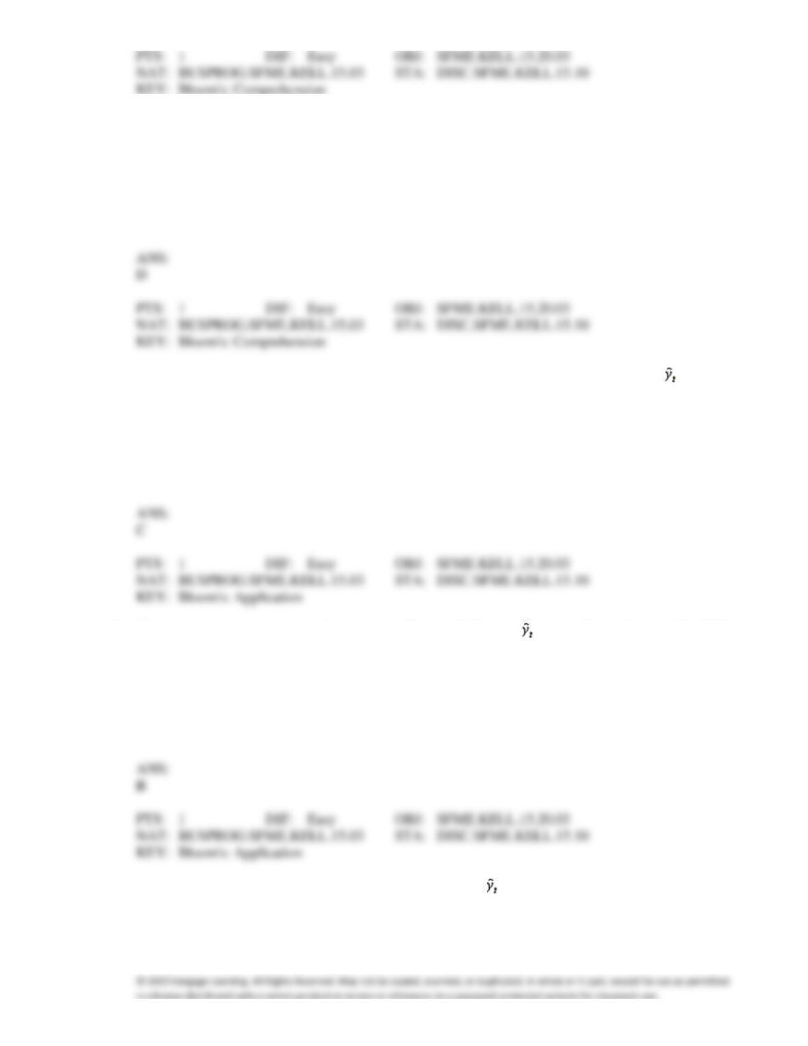
48. The trend equation for quarter sales data (in millions of dollars) for 2011-2015 is given by = 6.8 +
1.2t, where t = 1 for the first quarter of 2011. The seasonal index for the third quarter of 2008 is 1.25.
The forecasted sales’ value for the third quarter of 2016 is:
a.
34.40
b.
27.52
c.
43.00
d.
35.65
49. The trend equation for annual sales data (in millions of dollars) is = 65 + 2.5t, where t = 1 for 2011.
The monthly seasonal index for December is 0.97. The forecasted sales’ value for December of 2020
is:
a.
90.0
b.
7.28
c.
7.50
d.
7.69
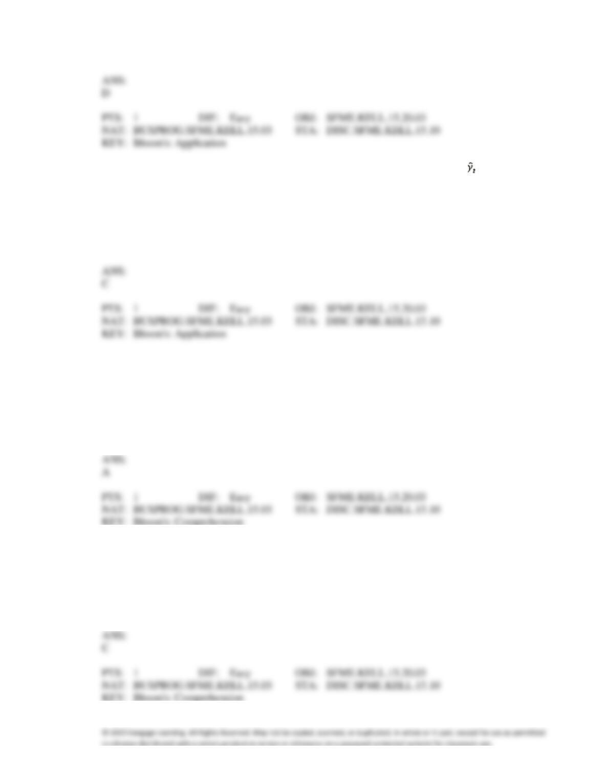
50. The results of a quadratic model fit to time series data were = 7.5 − 0.25t + 3.5t2, where t = 1 for
2011. The forecasted value for 2018 is:
a.
3.25
b.
10.75
c.
28.0
d.
229.5
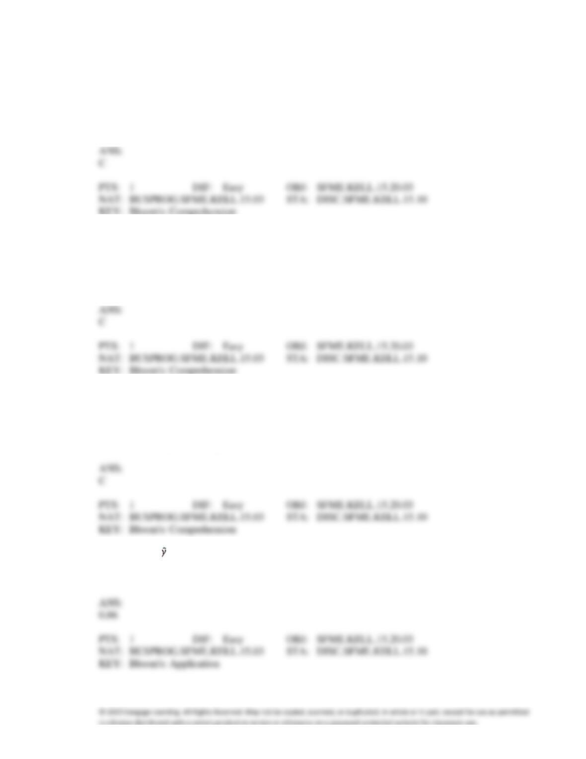
51. The regression trend line for annual energy consumption for 2000-2020 is given by = 70 + 0.50t,
where t = 1 for 2000. If the annual energy consumption for 2015 was 72.5, then the percentage of trend
for 2015 was:
a.
93.548
b.
106.897
c.
92.949
d.
107.586
52. In determining weekly seasonal indexes for gas consumption, the sum of the 52 means for gas
consumption as a percentage of the moving average is 5050. To get the seasonal indexes, each weekly
mean is to be multiplied by:
a.
5200 / 5050
b.
(5200 + 5050) / 52
c.
(5050 + 52) / 5200
d.
5050 / 5200
53. Which of the following models might be appropriate to describe a new product that has experienced a
rapid early growth rate followed by the inevitable leveling off?
a.
Autoregressive model
b.
Linear model for long-term trend
c.
Quadratic model for long-term trend
d.
All of these choices are true
54. Which of the following statements is true?
a.
In trend analysis, the independent variable is time only if the equation is linear.
b.
The number of time periods in centered moving average is always even.
c.
If the seasonal index for December sales is 120, this means that December sales tend to be
120% as high as the “average” month.
d.
The cyclical component of a time series refers to repeating patterns that have a period of a
year or less.
55. A model that can be used to make predictions about long term future values of a time series is
a.
linear trend model
b.
quadratic trend model
c.
both a and b
d.
neither a nor b
56. The method of least squares is used on time-series data for
a.
eliminating irregular movements
b.
deseasonalizing the data
c.
obtaining the trend equation
d.
exponentially smoothing a series
57. The trend line = 0.75 + 0.005t was calculated from quarterly data for 2000-2004, where t = 1 for the
first quarter of 2000. The trend value for the second quarter of the year 2005 is
____________________.