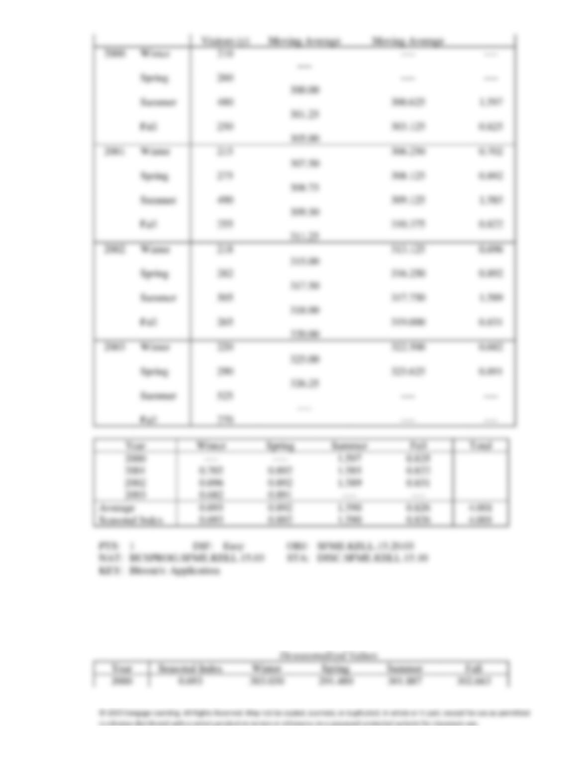
92. {The Pyramids of Giza Narrative} Use the seasonal indexes computed in the previous question to
deseasonalize the original time series data, and plot the deseasonalized time series.
ANS:
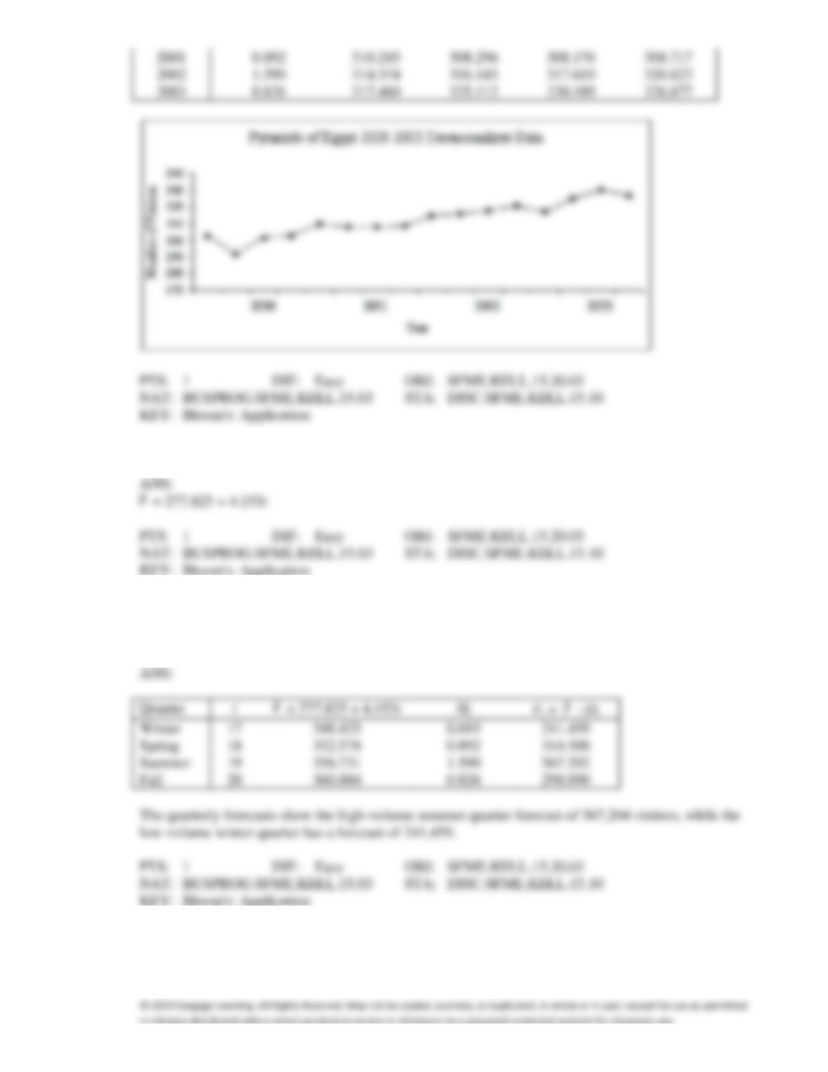
93. {The Pyramids of Giza Narrative} Use regression analysis to develop the trend line.
94. {The Pyramids of Giza Narrative} Use the seasonal indexes and the linear trend calculated in the
previous questions to forecast the number of visitors in the next four quarters and describe the seasonal
fluctuations in the number of visitors.
95. A time series is shown in the table below.
Time Period
yt
Time Period
yt
1
5
5
50
2
8
6
85
3
14
7
135
4
25
8
190
a.
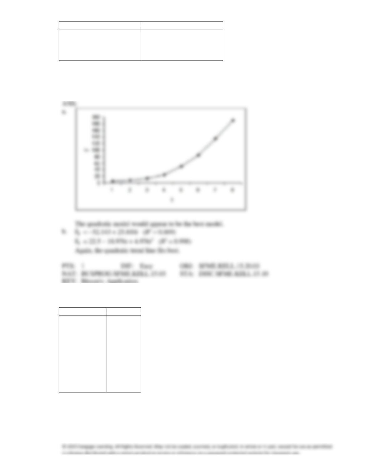
Plot the time series. Would the linear or quadratic model fit better?
b.
Use the regression technique to calculate the linear trend line and the quadratic trend line.
Which model fits better?
The quadratic model would appear to be the best model.
Again, the quadratic trend line fits best.
96. A time series is shown in the table below:
Time Period
yt
1
48
2
50
3
46
4
42
5
40
6
32
7
34
8
26
9
21
10
13
a.
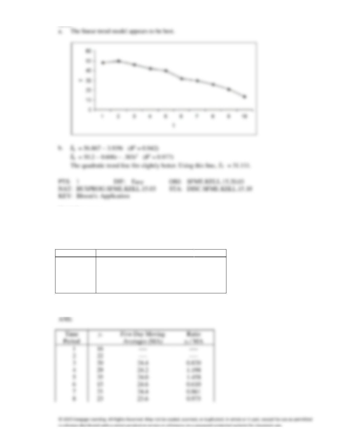
Plot the time series to determine which of the trend models appears to fit better.
b.
Use the regression technique to calculate the linear trend line and the quadratic trend line.
Which line fits better? Use the best model to forecast the value of y for time period 7.
ANS:
The linear trend model appears to be best.
Hotel Occupancy
A small hotel has recorded the number of rooms occupied during weekdays over a period of four
weeks as is shown in the table below:
Week
Day
1
2
3
4
Monday
16
15
18
21
Tuesday
22
21
20
25
Wednesday
20
23
20
24
Thursday
29
28
32
28
Friday
35
31
29
36
97. {Hotel Occupancy Narrative} Calculate the seasonal (daily) indexes.
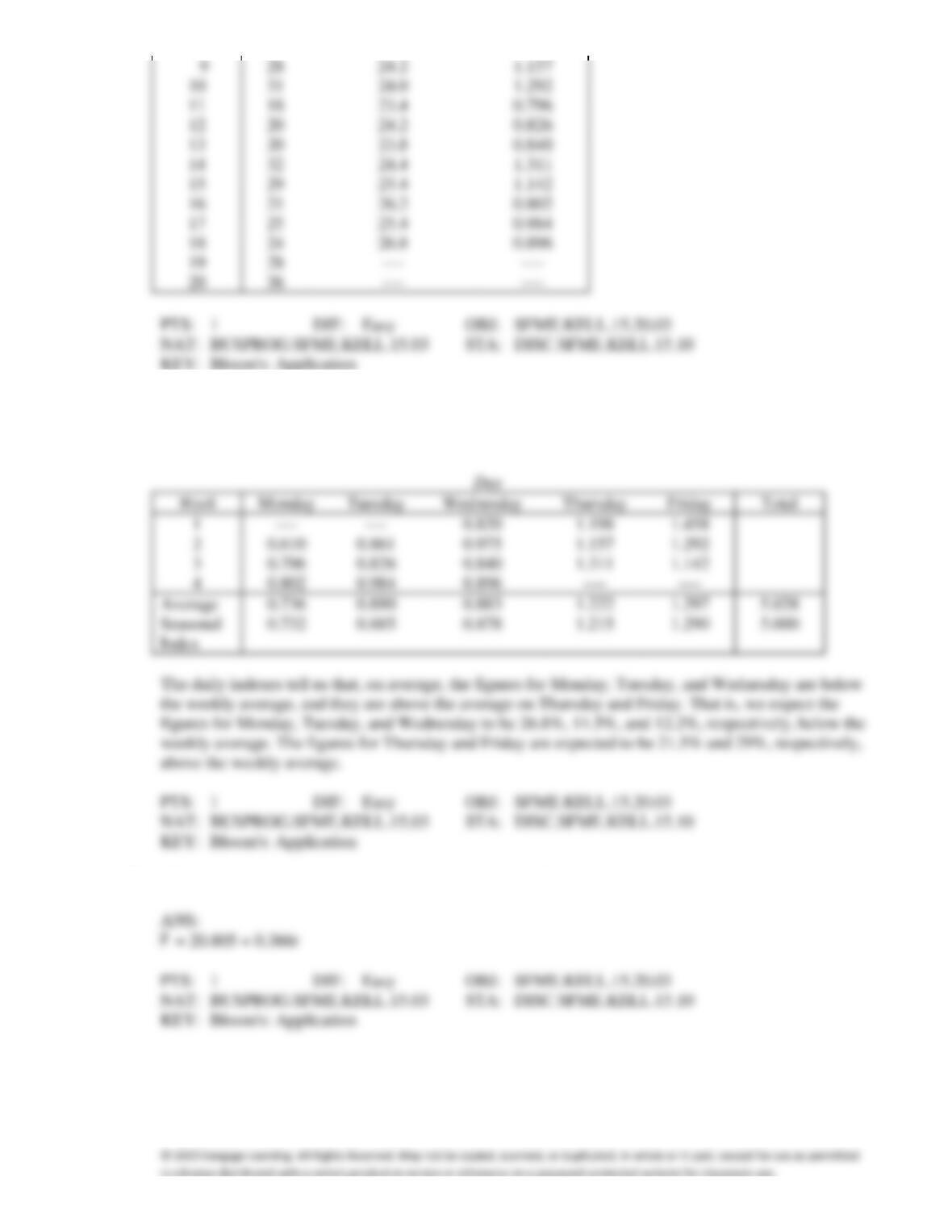
98. {Hotel Occupancy Narrative} What do the daily indexes tell us?
ANS:
99. {Hotel Occupancy Narrative} Find the regression trend line.
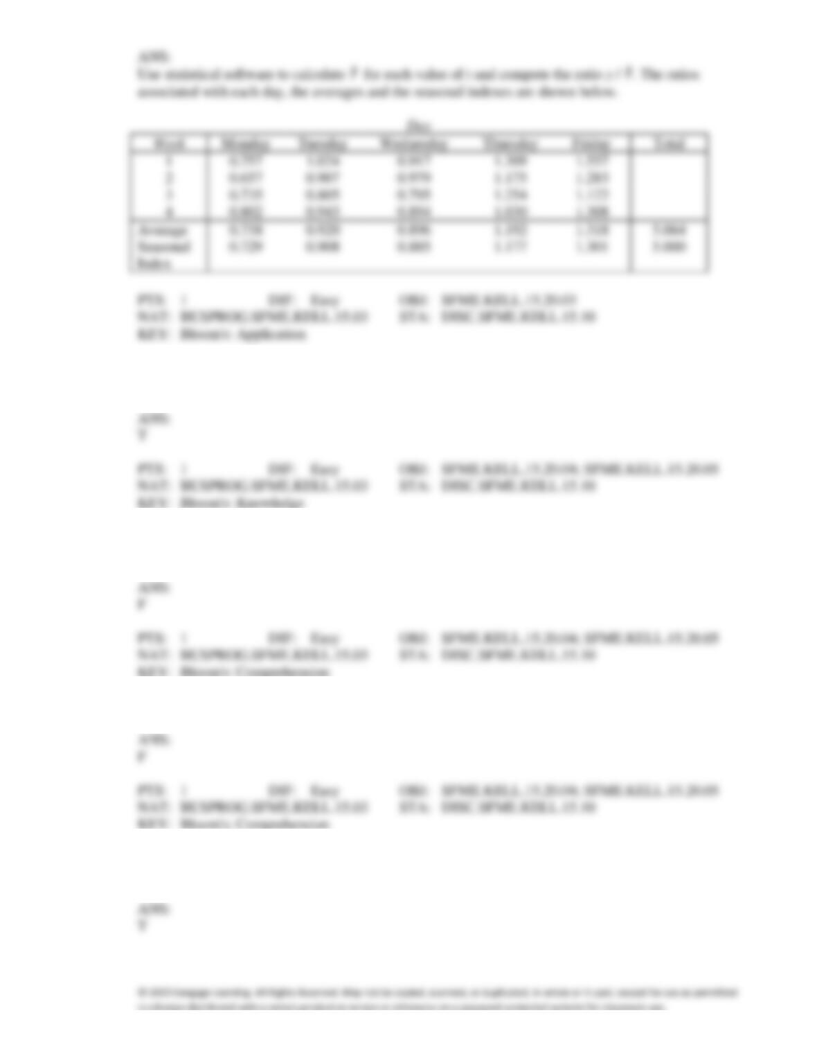
100. {Hotel Occupancy Narrative} Calculate the seasonal indexes, based on the regression trend line
developed in the previous question.
101. The most commonly used measures of forecast accuracy are the mean absolute deviation (MAD) and
the sum of squares for forecast error (SSE).
102. The mean absolute deviation averages the absolute differences between the actual values of the time
series at time t and the forecast values at time t + 1.
103. The mean absolute deviation is the summation of the residuals divided by the sample size.
104. The mean absolute deviation is a measure of the average of the absolute discrepancies between the
actual and the fitted values in a given time series.
105. If the time series is composed of seasonal variation and long-term trend, we can use seasonal indexes
and the regression equation to forecast.
106. If the time series displays a gradual or no trend and no evidence of seasonal variation, exponential
smoothing is not an effective as a forecasting method.
107. If there is no obvious trend or seasonality in the time series data, and we believe that there is a
correlation between consecutive residuals, the autoregressive model may be most effective as a
forecasting technique.
108. If we have 5 years of monthly observations, we may use the first four years to develop several
competing forecasting models, and then use them to forecast the fifth year. Since we know the actual
values in the fifth year, we can choose the technique that results in the most accurate forecast using
either the mean absolute deviation (MAD) or the sum of squares for forecast error (SSE).
109. The mean absolute deviation averages the absolute differences between the actual values of the time
series at time t and the forecast values at time:
a.
t + 1
b.
t
c.
t − 1
d.
t − 2
110. Which method would you recommend to your statistics professor in selecting the appropriate
forecasting model if avoiding large errors is extremely important to him or her?
a.
Mean absolute deviation (MAD)
b.
Sum of squares for forecast error (SSE)
c.
Either a or b
d.
Neither a nor b
111. The most commonly used measures of forecast accuracy are the:
a.
mean absolute deviation and the sum of squares for forecast errors
b.
sum of squares for forecast error and seasonal indexes
c.
seasonal indexes and the percentage of trend
d.
all of these choices are correct
112. The mean absolute deviation (MAD) and the sum of squares for forecast error (SSE) are the most
commonly used measures of forecast accuracy. The model that forecasts the data best will usually
have the:
a.
lowest MAD and highest SSE
b.
highest MAD and lowest SSE
c.
lowest MAD and SSE
d.
highest MAD and SSE
113. One measure of the accuracy of a forecasting model is the:
a.
deseasonalized time series
b.
four-period moving averages
c.
mean absolute deviation
d.
smoothing constant
114. To assess the adequacy of a forecasting model, one measure that is often used is the
a.
quadratic trend analysis
b.
mean absolute deviation
c.
exponential smoothing
d.
moving averages
115. The following is the list of mean absolute deviation (MAD) statistics for each of the models you have
estimated from time-series data:
Model
MAD
Linear Trend
1.38
Quadratic Trend
1.22
Exponential Trend
1.39
Autoregressive(2)
0.71
Based on the MAD criterion, the most appropriate model is
a.
linear trend
b.
quadratic trend
c.
exponential trend
d.
autoregressive(2)
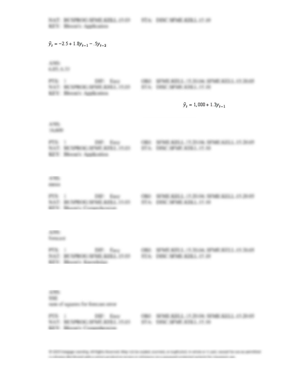
116. An estimated second-order autoregressive model for average mortgage rate is:
. If the average mortgage rate in 2004 was 6.5 and in 2011 was 6.0, the
forecast for 2013 is ____________________.
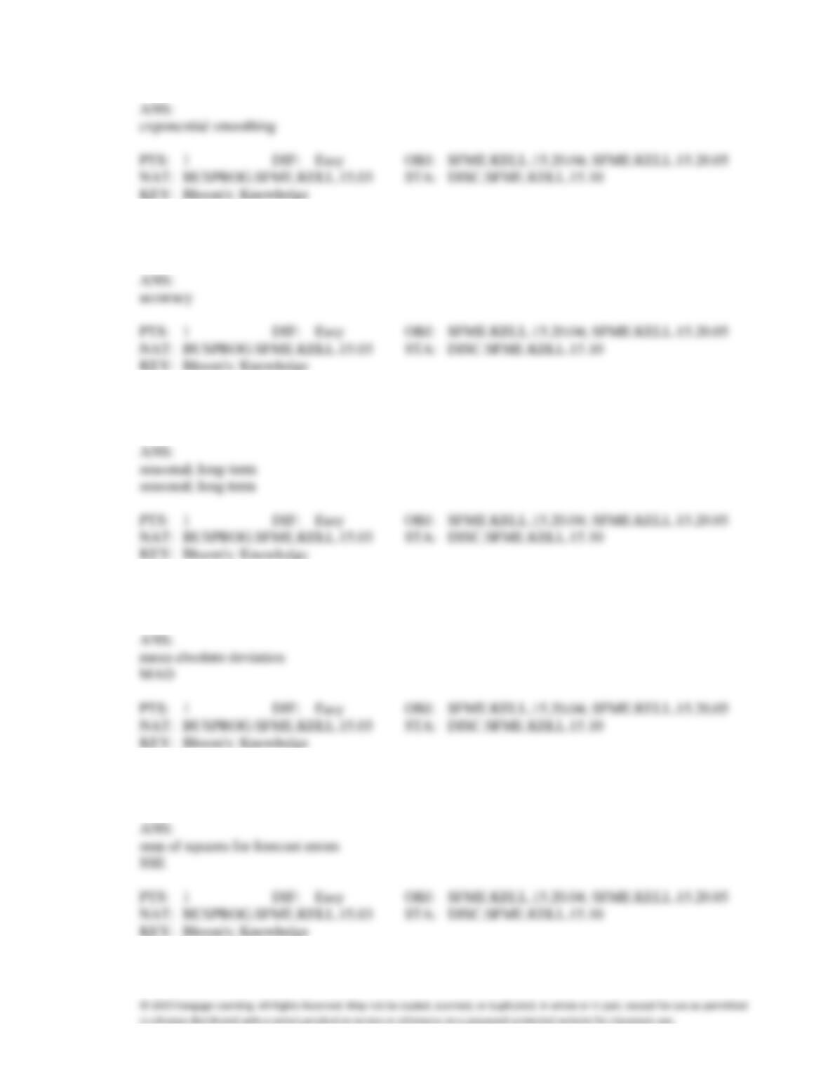
117. An estimated second-order autoregressive model for average mortgage rate is:
. If the average mortgage rate in 2003 was 7.0, and in 2002 was 6.5, the
forecast for 2004 is ____________________, and for 2005 is ____________________.
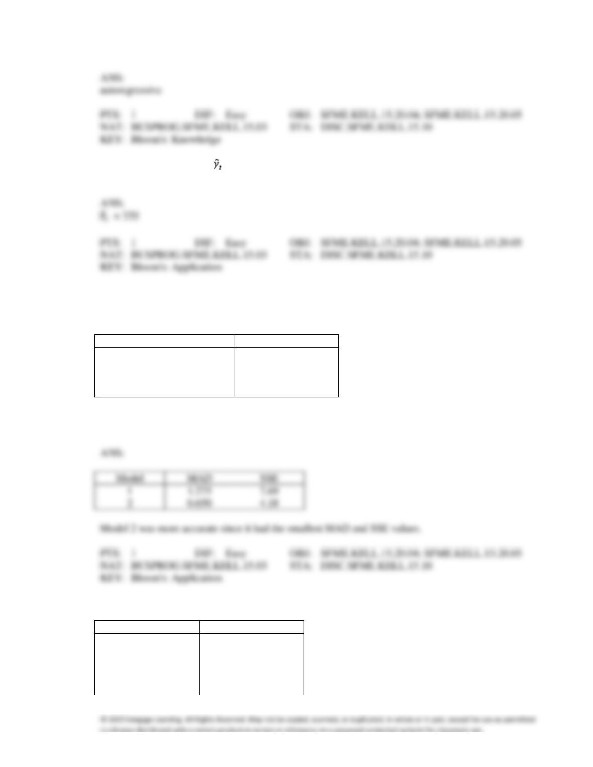
118. An estimated first-order autoregressive model for stock sales is: . If sales in 2011
were 12,000, the forecast of sales for 2012 is ____________________.
119. MAD stands for ____________________ absolute deviation.
120. MAD averages the absolute differences between the actual and ____________________ values.
121. If avoiding large errors is important, ____________________ should be used because it penalizes
large deviations more heavily than does MAD.
122. If a time series displays a gradual or no trend and no evidence of seasonal variation,
____________________ can be effective as a forecasting method.
123. It must be understood that the ____________________ of a forecast decreases rapidly for predictions
more than one time period into the future.
124. If the time series is composed of ____________________ variation and ____________________
trend, we can use seasonal indexes and the regression equation to forecast.
125. The most commonly used measures of forecast accuracy are ____________________ and the sum of
squares for forecast errors (SSE).
126. The most commonly used measures of forecast accuracy are mean absolute deviation (MAD) and the
____________________.
127. If there is no obvious trend or seasonality and we believe that there is a correlation between
consecutive residuals, the ____________________ model may be most effective.
128. The autoregressive model = 200 + 15yt − 1 was developed from a time series. Forecast the next
value of the time series if the last observation was 8.
129. Two forecasting models were used to predict the future values of a time series. These are shown in the
accompanying table, together with the actual values.
Forecast Value Ft
Actual Value yt
Model 1
Model 2
9.0
7.7
7.6
7.8
8.1
8.2
7.0
8.5
8.9
9.6
9.0
11.0
Compute the mean absolute deviation (MAD) and sum of squares for forecast (SSE) for each model to
determine which was more accurate.
130. The actual and forecast values of a time series are shown below.
Actual Values yt
Forecast Values Ft
135
140
162
165
155
150
182
191
174
168
194
190
233
220
280
240
a.
Calculate the mean absolute deviation (MAD).
b.
Calculate the sum of squares for forecast error (SSE)
131. The actual and forecast values of a time series are shown below.
Actual Values yt
Forecast Values Ft
2325
2330
2555
2595
2835
2860
3185
3125
3510
3390
a.
Calculate the mean absolute deviation (MAD).
b.
Calculate the sum of squares for forecast error (SSE)
132. A time series for the years 1996-2001 is shown below.
Year
yt
1996
125
1997
115
1998
120
1999
126
2000
140
2001
122
The forecasts for the years 2002-2004 with three smoothing constant values are:
With w = .2, F2002 = F2003 = F2004 = 125.60
With w = .5, F2002 = F2003 = F2004 = 126.75
With w = .6, F2002 = F2003 = F2004 = 126.55
Compare each of the three sets of forecasts with the actual values for 2002-2004 given in the
accompanying table, and compute the mean absolute deviation (MAD) for each model. Which model
is best?
Year
yt
2002
130
2003
125
2004
135