KEY: Bloom’s: Application
19. {Student’s Final Grade Narrative} Interpret the coefficient b1.
20. {Student’s Final Grade Narrative} Interpret the coefficient b2.
21. {Student’s Final Grade Narrative} Interpret the coefficient b3.
Real Estate Builder
A real estate builder wishes to determine how house size is influenced by family income, family size,
and education of the head of household. House size is measured in hundreds of square feet, income is
measured in thousands of dollars, and education is measured in years. A partial computer output is
shown below.
SUMMARY OUTPUT
Regression Statistics
Multiple R
0.865
R Square
0.748
Adjusted R Square
0.726
Standard Error
5.195
Observations
50
ANOVA
df
SS
MS
F
Signif F
Regression
3605.7736
901.4434
0.0001
Residual
1214.2264
26.9828
Total
49
4820.0000
Coeff.
St. Error
t Stat
P-value
Intercept
−1.6335
5.8078
−0.281
0.7798
Family Income
0.4485
0.1137
3.9545
0.0003
Family Size
4.2615
0.8062
5.286
0.0001
Education
−0.6517
0.4319
−1.509
0.1383
22. {Real Estate Builder Narrative} What percentage of the variability in house size is explained by this
model?
23. {Real Estate Builder Narrative} Interpret the value of the Adjusted R-Square.
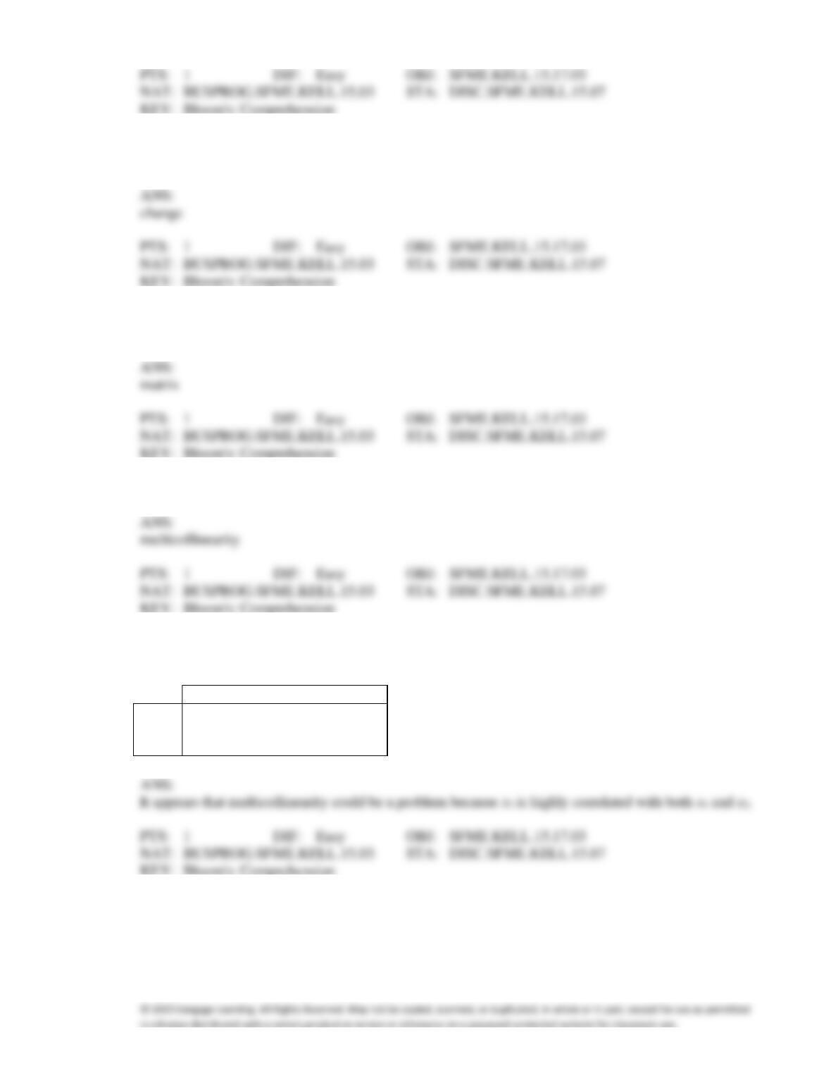
24. {Real Estate Builder Narrative} Which of the independent variables in the model are significant at the
2% level?
25. {Real Estate Builder Narrative} Which of the following values for the level of significance is the
smallest for which all explanatory variables are significant individually:
= .01, .05, .10, or .15?
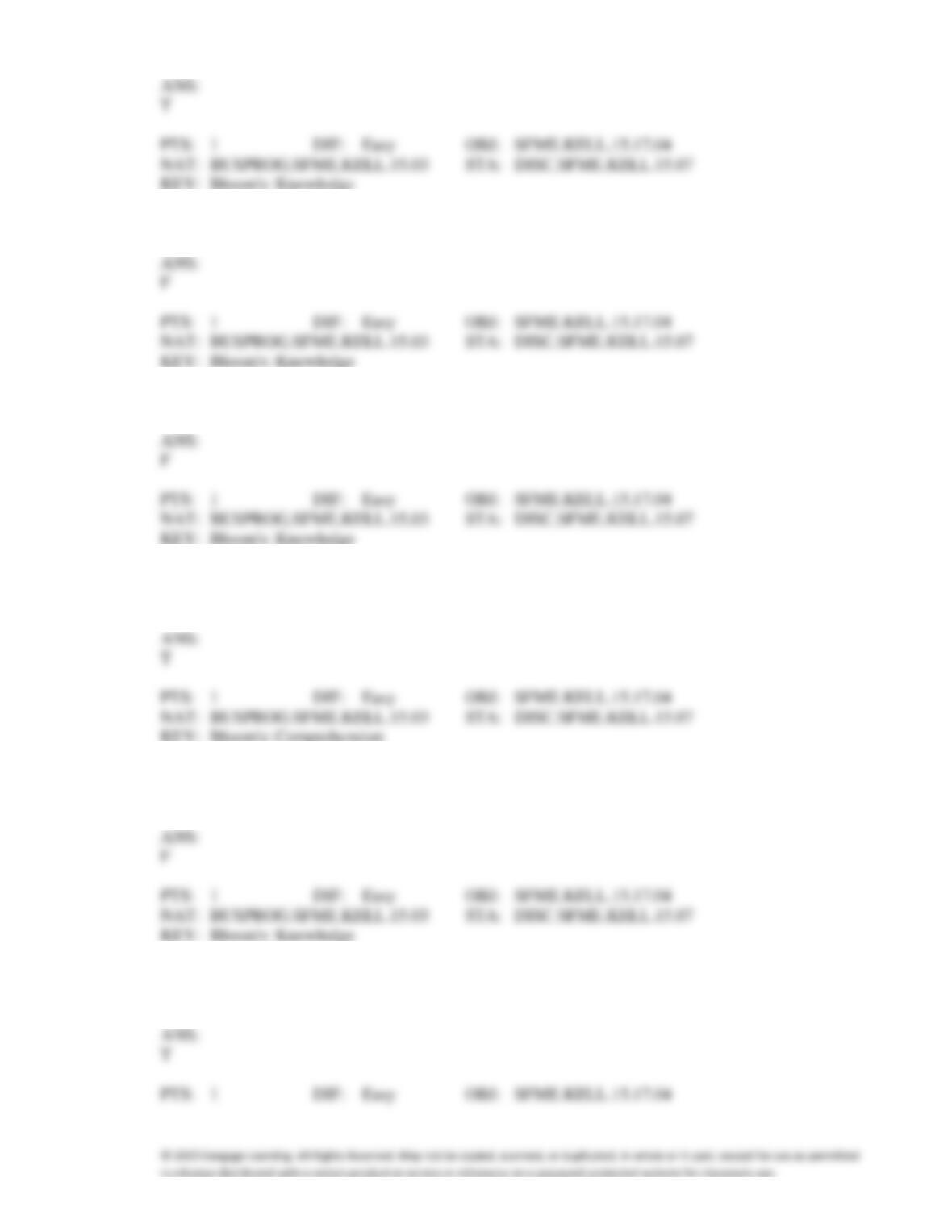
26. {Real Estate Builder Narrative} When the builder used a simple linear regression model with house
size as the dependent variable and education as the independent variable, he obtained an R-square
value of 23.0%. What additional percentage of the total variation in house size has been explained by
including family size and income in the multiple regression?
27. {Real Estate Builder Narrative} Which of the following values for the level of significance is the
smallest for which at least two explanatory variables are significant individually:
= .01, .05, .10, and
.15?
28. {Real Estate Builder Narrative} Which of the following values for the level of significance is the
smallest for which the regression model as a whole is significant:
= .00005, .001, .01, and .05?
29. {Real Estate Builder Narrative} What is the predicted house size for an individual earning an annual
income of $40,000, having a family size of 4, and having 13 years of education?
30. {Real Estate Builder Narrative} What minimum annual income would an individual with a family size
of 4 and 16 years of education need to attain a predicted 10,000 square foot home?
31. {Real Estate Builder Narrative} What minimum annual income would an individual with a family size
of 9 and 10 years of education need to attain a predicted 5,000 square foot home?
32. {Real Estate Builder Narrative} One individual in the sample had an annual income of $100,000, a
family size of 10, and an education of 16 years. This individual owned a home with an area of 7,000
square feet. What is the residual (in hundreds of square feet) for this data point?
33. {Real Estate Builder Narrative} One individual in the sample had an annual income of $10,000, a
family size of 1, and an education of 8 years. This individual owned a home with an area of 1,000
square fee (House = 10.00). What is the residual (in hundreds of square feet) for this data point?
34. {Real Estate Builder Narrative} Suppose the builder wants to test whether the coefficient on income is
significantly different from 0. What is the value of the relevant t-statistic?
35. {Real Estate Builder Narrative} At the 0.01 level of significance, what conclusion should the builder
draw regarding the inclusion of income in the regression model?
36. {Real Estate Builder Narrative} Suppose the builder wants to test whether the coefficient on education
is significantly different from 0. What is the value of the relevant t-statistic?
37. {Real Estate Builder Narrative} What is the value of the calculated F-test statistic that is missing from
the output for testing whether the whole regression model is significant?
38. {Real Estate Builder Narrative} At the 0.01 level of significance, what conclusion should the builder
draw regarding the inclusion of education in the regression model?
39. {Real Estate Builder Narrative} What are the regression degrees of freedom that are missing from the
output?
40. {Real Estate Builder Narrative} What are the residual degrees of freedom that are missing from the
output?
41. {Real Estate Builder Narrative} What are the numerator and denominator degrees of freedom for the
F-statistic?
42. Multicollinearity is present if the dependent variable is linearly related to one of the explanatory
variables.
43. Multicollinearity affects the t-tests of the individual coefficients as well as the F-test in the analysis of
variance for regression because the F-test combines the t-tests into a single test.
44. Because of multicollinearity, the t–tests of the individual coefficients may indicate that some
independent variables are not linearly related to the dependent variable, when in fact they are.
45. Multicollinearity is present when there is a high degree of correlation between the dependent variable
and any of the independent variables.
46. One of the consequences of multicollinearity in multiple regression is biased estimates on the slope
coefficients.
ANS:
47. Multicollinearity is a situation in which two or more of the independent variables are highly correlated
with each other.
48. Multicollinearity is present when there is a high degree of correlation between the independent
variables included in the regression model.
49. One of the consequences of multicollinearity in multiple regression is inflated standard errors in some
or all of the estimated slope coefficients.
50. The parameter estimates are biased when multicollinearity is present in a multiple regression equation.
51. Multicollinearity will result in excessively low standard errors of the parameter estimates reported in
the regression output.
52. Which of the following statements regarding multicollinearity is not true?
a.
It exists in virtually all multiple regression models.
b.
It is also called collinearity and intercorrelation.
c.
It is a condition that exists when the independent variables are highly correlated with the
dependent variable.
d.
All of these choices are true.
53. When the independent variables are correlated with one another in a multiple regression analysis, this
condition is called:
a.
heteroscedasticity.
b.
homoscedasticity.
c.
multicollinearity.
d.
None of these choices.
54. The problem of multicollinearity arises when the:
a.
dependent variables are highly correlated with one another.
b.
independent variables are highly correlated with one another.
c.
independent variables are highly correlated with the dependent variable.
d.
None of these choices.
55. If multicollinearity exists among the independent variables included in a multiple regression model,
then:
a.
the regression coefficients will be difficult to interpret.
b.
the standard errors of the regression coefficients for the correlated independent variables
will increase.
c.
one or more of the coefficients may have the wrong sign.
d.
All of these choices are true.
56. If a group of independent variables are not significant individually but are significant as a group at a
specified level of significance, this is most likely due to:
a.
heteroscedasticity.
b.
an error in the analysis.
c.
multicollinearity.
d.
None of these choices.
57. ____________________ is a condition that exists when independent variables are correlated with one
another.
58. An adverse effect of multicollinearity is that the estimated regression coefficients of the independent
variables that are correlated tend to have large sampling ____________________.
59. One clue to the presence of multicollinearity is an independent variable known to be an important
predictor that ends up having a regression coefficient that is not ____________________.
60. There are several clues to the presence of multicollinearity. One clue is when a regression coefficient
exhibits the wrong ____________________.
61. There are several clues to the presence of multicollinearity. One clue is when an independent variable
is added or deleted, the regression coefficients for the other variables ____________________.
62. A practical way to identify multicollinearity is through the examination of a correlation
____________________ that shows the correlations of each variable with each of the other variables.
63. A high correlation between two independent variables is an indication of ____________________.
64. Three predictor variables are being considered for use in a linear regression model. Given the
correlation matrix below, does it appear that multicollinearity could be a problem?
x1
x2
x3
x1
1.000
x2
0.025
1.000
x3
0.968
0.897
1.000
65. Discuss two indicators that can be found in an analysis that suggest multicollinearity is present.
ANS:
66. How do you go about checking for multicollinearity?
67. The Durbin-Watson d statistic is used to check the assumption of normality.
68. The Durbin-Watson test allows the statistics practitioner to determine whether there is evidence of
first-order autocorrelation.
69. The Durbin-Watson statistic, d, is defined as , where ei is the residual at
time period i.
70. The range of the values of the Durbin-Watson statistic, d, is 0 d 4.
71. Small values of the Durbin-Watson statistic d (d < 2) indicate a negative first-order autocorrelation.
72. Large values of the Durbin-Watson statistic d (d > 2) indicate a positive first-order autocorrelation.
73. If the value of the Durbin-Watson statistic, d, satisfies the inequality dL d dU, where dL and dU are
the critical values for d, then the test for positive first-order autocorrelation is inconclusive.
74. If the value of the Durbin-Watson test statistic, d, satisfies the inequality d > 4 − dL, we conclude that
positive first-order autocorrelation exists.
75. If the value of the Durbin-Watson test statistic, d, satisfies the inequalities d < dL or d > 4 − dL, where
dL and dU are the critical values of d, we conclude that autocorrelation exists.
76. If the Durbin-Watson statistic has a value close to 0, which assumption is violated?
a.
Homoscedasticity.
b.
Normality of the errors.
c.
Independence of errors.
d.
None of these choices.
77. If the Durbin-Watson statistic d has values smaller than 2, this indicates
a.
a positive first-order autocorrelation
b.
a negative first-order autocorrelation
c.
no first-order autocorrelation at all
d.
None of these choices.
78. If the Durbin-Watson statistic, d, has values greater than 2, this indicates
a.
a positive first-order autocorrelation
b.
a negative first-order autocorrelation
c.
no first-order autocorrelation at all
d.
None of these choices.
79. If the Durbin-Watson statistic has a value close to 4, which assumption is violated?
a.
Homoscedasticity
b.
Normality of the errors
c.
Independence of errors
d.
None of these choices.
80. The range of the values of the Durbin-Watson statistic d is:
a.
−4 d 4
b.
−2 d 2
c.
0 d 2
d.
0 d 4
81. If the residuals in a regression analysis of time ordered data are not correlated, the value of the
Durbin-Watson d statistic should be near ____________________.
82. If the value of the Durbin-Watson statistic d is small (d < 2), this indicates a(n)
____________________ (positive/negative) first-order autocorrelation exists.
83. If the value of the Durbin-Watson statistic d is large (d > 2), this indicates a(n)
____________________ (positive/negative) first-order autocorrelation exists.
84. To use the Durbin-Watson test to test for positive first-order autocorrelation, the null hypothesis will
be H0: ____________________ (there is/there is no) first-order autocorrelation.
85. To use the Durbin-Watson test to test for negative first-order autocorrelation, the null hypothesis will
be H0: ____________________ (there is/there is no) first-order autocorrelation.
86. The range of the values of the Durbin-Watson statistic d is ____________________.
87. Given that the Durbin-Watson test is conducted to test for positive first-order autocorrelation with
=
.05, n = 20, and there are two independent variables in the model, the critical values for the test are dL
= __________ and dU = __________, respectively.
88. Test the hypotheses: H0: There is no first-order autocorrelation vs. H1: There is negative first-order
autocorrelation, given that: Durbin-Watson Statistic d = 1.75, n = 20, k = 2, and
= 0.01.
89. Test the hypotheses H0: There is no first-order autocorrelation vs. H1: There is positive first-order
autocorrelation, given that: Durbin-Watson Statistic d = 1.12, n = 45, k = 5, and
= 0.05.
90. Test the hypotheses H0: no first-order autocorrelation vs. H1: first-order autocorrelation, given that:
Durbin-Watson Statistic d = 1.89, n = 28, k = 3, and
= 0.01.