CHAPTER 16B: SIMPLE LINEAR REGRESSION AND CORRELATION
TRUE/FALSE
1. Data that exhibit an autocorrelation effect violate the regression assumption of independence.
2. We standardize residuals by subtracting their mean and dividing by their variance.
3. An outlier is an observation that is unusually small or unusually large.
4. We check for normality by drawing a pie chart of the residuals.
5. One method of diagnosing heteroscedasticity is to plot the residuals against the predicted values of y,
then look for a change in the spread of the plotted values.
6. The spread in the residuals should increase as the predicted value of y increases.
7. The plot of residuals vs. predicted values should show no patterns if the conditions of a regression
analysis are met.
8. If the plot of the residuals vs. the predicted values resembles a straight line with non-zero slope, then
the regression line fits well.
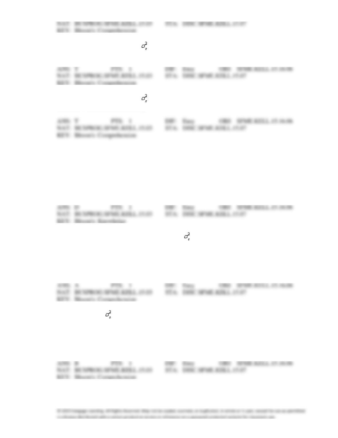
9. The variance of the error variable is required to be constant. When this requirement is violated, the
condition is called heteroscedasticity.
10. The variance of the error variable is required to be constant. When this requirement is satisfied, the
condition is called homoscedasticity.
MULTIPLE CHOICE
1. The standardized residual is defined as:
a.
residual multiplied by the square root of the standard error of estimate.
b.
residual multiplied by the standard error of estimate.
c.
residual divided by the square of the standard error of estimate.
d.
residual divided by the standard error of estimate.
2. The least squares method requires that the variance of the error variable
is a constant no matter
what the value of x is. When this requirement is violated, the condition is called:
a.
heteroscedasticity.
b.
homoscedasticity.
c.
influential observation.
d.
non-independence of
.
3. When the variance of the error variable
is a constant no matter what the value of x is, this
condition is called:
a.
heterocausality.
b.
homoscedasticity.
c.
homocausality.
d.
heteroscedasticity.
4. If the plot of the residuals is fan shaped, which assumption of regression analysis (if any) is violated?
a.
No assumptions are violated.
b.
Independence of errors
c.
Homoscedasticity
d.
Normality
COMPLETION
1. If you take the residuals, subtract their mean and divide by their standard deviation, the result is called
the ____________________ residuals.
2. We check for normality by drawing a(n) ____________________ of the residuals.
3. If the variance of the errors is constant for each predicted y value, the condition is called
____________________.
4. When the error variable does not have constant variance, this condition is called
____________________.
5. Error terms that are correlated over time are said to be ____________________.
6. Error terms that are autocorrelated ____________________ (are/are not) independent.
7. We can often detect autocorrelation by graphing the residuals against ____________________.
8. A(n) ____________________ is an observation that is unusually small or large.
9. If a single point has a large impact on the equation of the regression line, it is called a(n)
____________________ point.
SHORT ANSWER
Telemarketing Sales and Experience
The general manager of a telemarketing company believes that experience is the most important factor
in determining the level of success of a telemarketer. To examine this belief she records last month’s
sales (in $1,000s) and the years of experience of 10 randomly selected telemarketers. These data are
listed below.
Telemarketer
Years of Experience
Sales
1
0
7
2
2
9
3
10
20
4
3
15
5
8
18
6
5
14
7
12
20
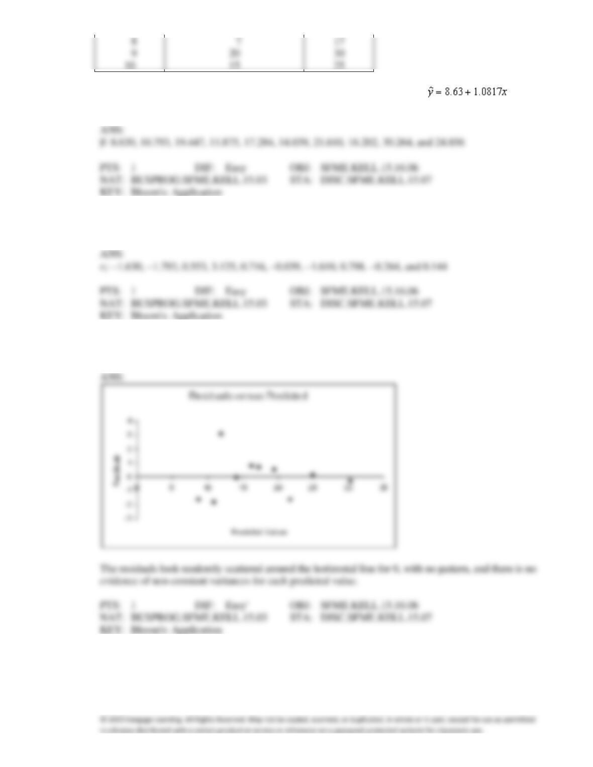
1. {Telemarketer Sales and Experience Narrative} Use the regression equation to
determine the predicted values of y.
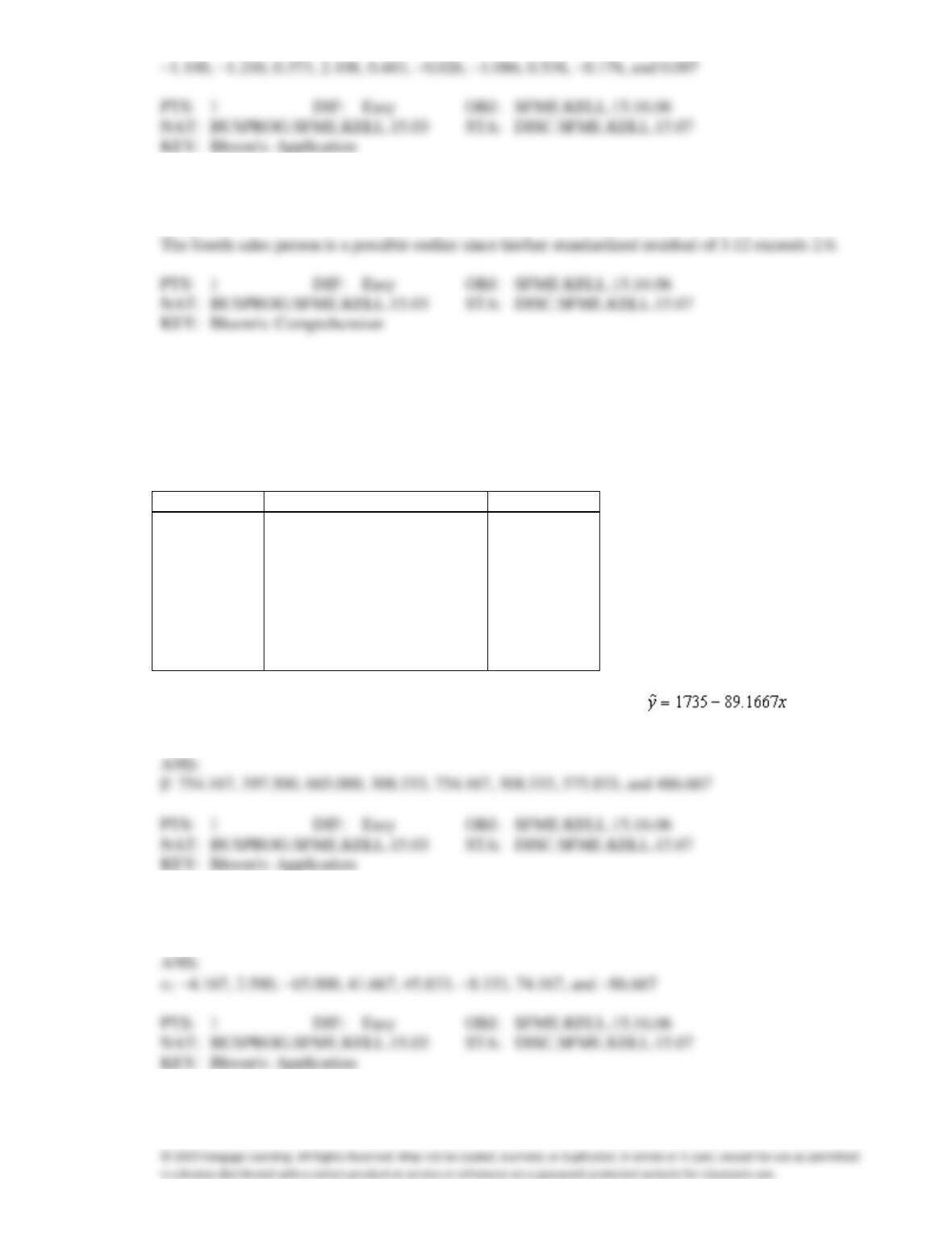
2. {Telemarketer Sales and Experience Narrative} Use the predicted and actual values of y to calculate
the residuals.
3. {Telemarketer Sales and Experience Narrative} Plot the residuals against the predicted values of y.
What does the graph tell you?
4. {Telemarketer Sales and Experience Narrative} Compute the standardized residuals.
ANS:
5. {Telemarketer Sales and Experience Narrative} Identify possible outliers.
ANS:
Game Winnings & Education
An ardent fan of television game shows has observed that, in general, the more educated the
contestant, the less money he or she wins. To test her belief she gathers data about the last eight
winners of her favorite game show. She records their winnings in dollars and the number of years of
education. The results are as follows.
Contestant
Years of Education
Winnings
1
11
750
2
15
400
3
12
600
4
16
350
5
11
800
6
16
300
7
13
650
8
14
400
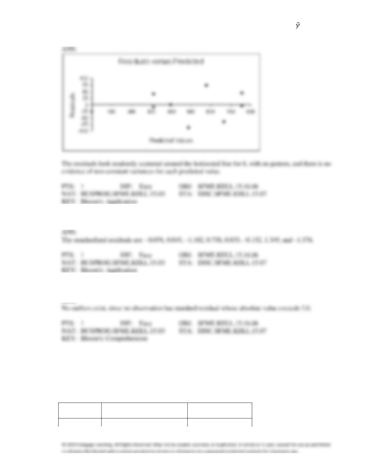
6. {Game Winnings & Education Narrative} Use the regression equation to
determine the predicted values of y.
7. {Game Winnings & Education Narrative} Use the predicted and actual values of y to calculate the
residuals.
8. {Game Winnings & Education Narrative} Plot the residuals against the predicted values . What does
the graph tell you?
9. {Game Winnings & Education Narrative} Compute the standardized residuals.
10. {Game Winnings & Education Narrative} Identify possible outliers.
Comedy Shows Revenues
A financier whose specialty is investing in comedy shows has observed that, in general, shows with
“big-name” stars seem to generate more revenue than those shows whose stars are less well known. To
examine his belief he records the gross revenue and the payment (in $ millions) given to the two
highest-paid comedians in the show for ten recently staged shows.
Show
Cost of Two Highest
Gross Revenue
Paid Comedian ($mil)
($mil)
1
5.3
48
2
7.2
65
3
1.3
18
4
1.8
20
5
3.5
31
6
2.6
26
7
8.0
73
8
2.4
23
9
4.5
39
10
6.7
58
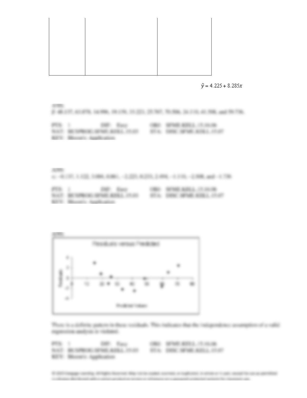
11. {Comedy Shows Revenues Narrative} Use the regression equation to determine
the predicted values of y.
12. {Comedy Shows Revenues Narrative} Use the predicted and actual values of y to calculate the
residuals.
13. {Comedy Shows Revenues Narrative} Plot the residuals against the predicted values of y. What does
the graph tell you?
Marc Anthony Concert
At a recent Marc Anthony concert, a survey was conducted that asked a random sample of 20 people
their age and how many concerts they have attended since the first of the year. The following data
were collected:
Age
62
57
40
49
67
54
43
65
54
41
Number of Concerts
6
5
4
3
5
5
2
6
3
1
Age
44
48
55
60
59
63
69
40
38
52
Number of Concerts
3
2
4
5
4
5
4
2
1
3
4.781
4.153
2.016
3.147
5.410
3.776
2.393
5.158
3.776
2.142
2.519
3.022
3.901
4.530
4.404
4.907
5.661
2.016
1.765
3.524
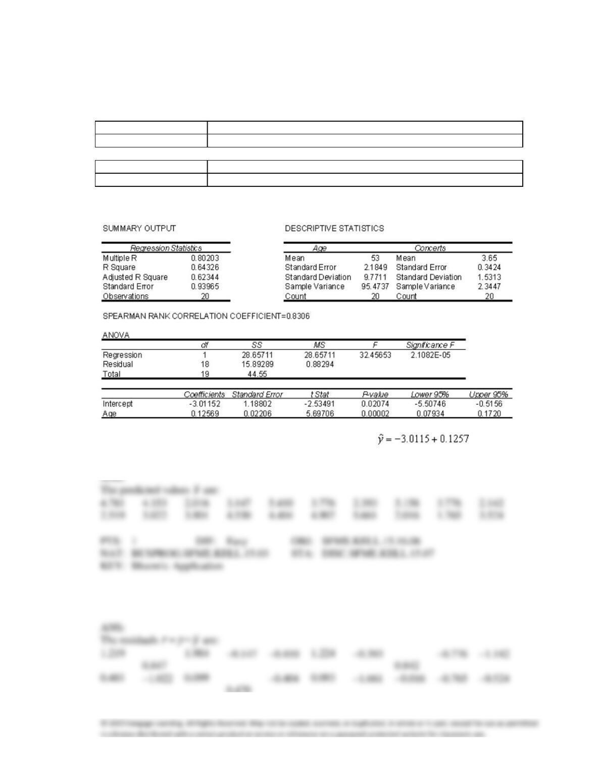
An Excel output follows:
14. {Marc Anthony Concert Narrative} Use the regression equation to determine the
predicted values of y.
0.847
0.842
15. {Marc Anthony Concert Narrative} Use the predicted values and the actual values of y to calculate the
residuals.
0.470
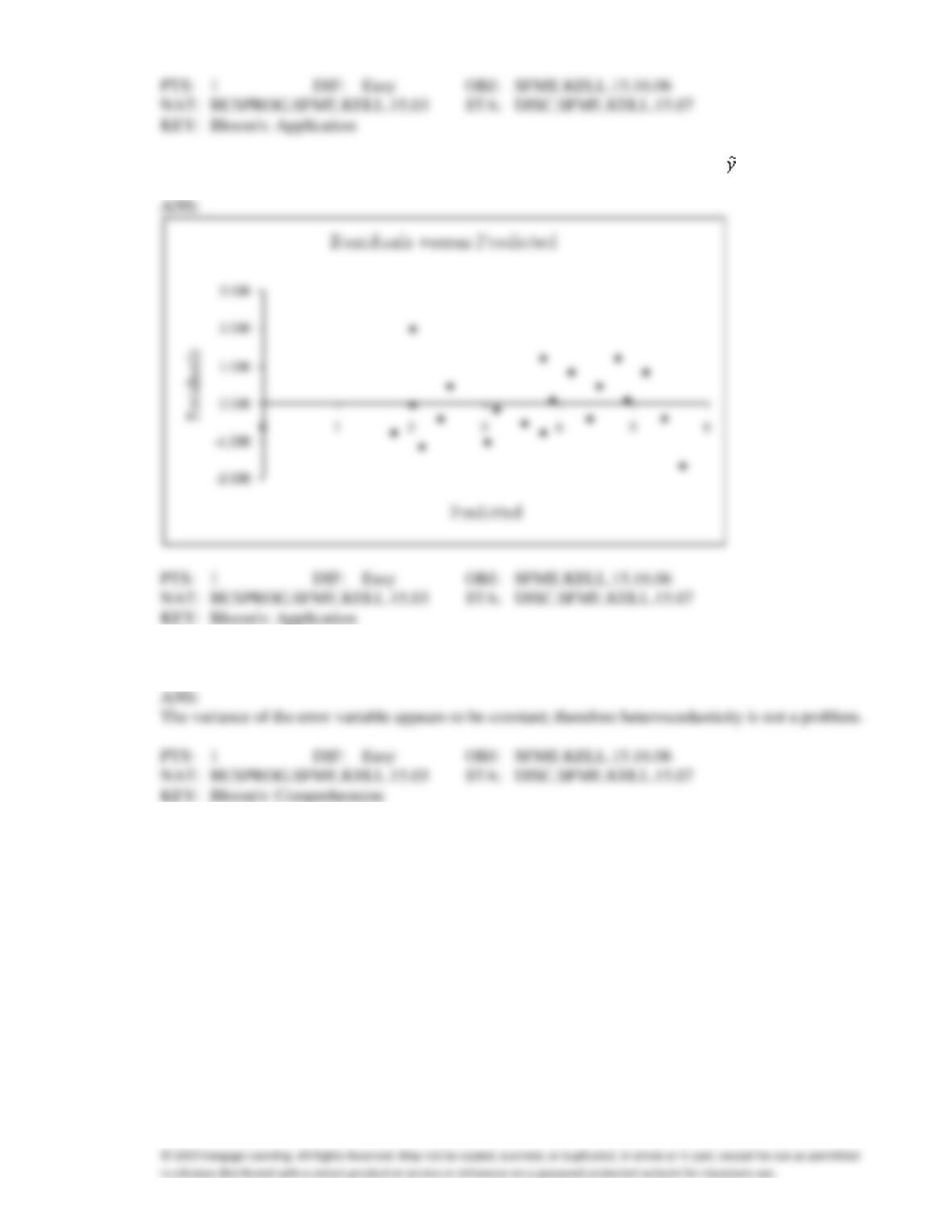
16. {Marc Anthony Concert Narrative} Plot the residuals against the predicted values .
17. {Marc Anthony Concert Narrative} Does it appear that heteroscedasticity is a problem? Explain.
18. {Marc Anthony Concert Narrative} Draw a histogram of the residuals.
ANS:
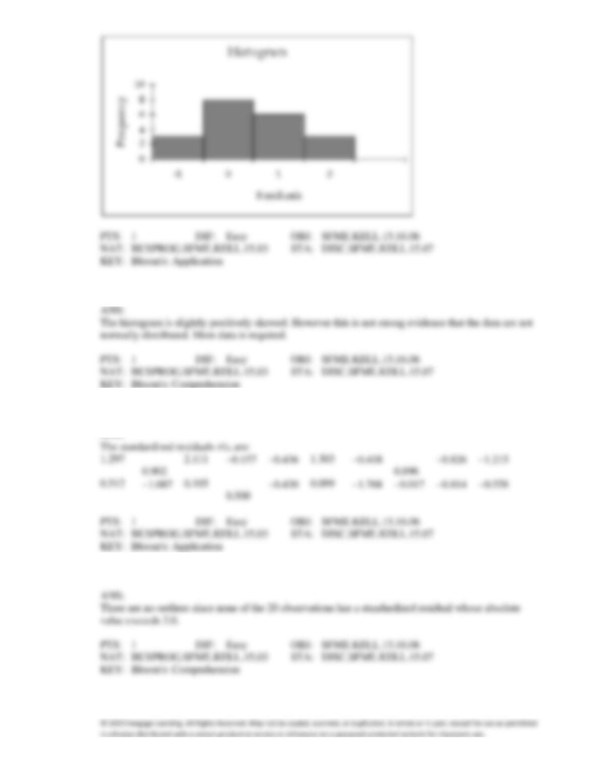
19. {Marc Anthony Concert Narrative} Does it appear that the errors are normally distributed? Explain.
20. {Marc Anthony Concert Narrative} Use the residuals to compute the standardized residuals.
ANS:
21. {Marc Anthony Concert Narrative} Identify possible outliers.
Oil Quality and Price
Quality of oil is measured in API gravity degrees—the higher the degrees API, the higher the quality.
The table shown below is produced by an expert in the field who believes that there is a relationship
between quality and price per barrel.
Oil degrees API
Price per barrel (in $)
27.0
12.02
28.5
12.04
30.8
12.32
31.3
12.27
31.9
12.49
34.5
12.70
34.0
12.80
34.7
13.00
37.0
13.00
41.0
13.17
41.0
13.19
38.8
13.22
39.3
13.27
A partial Minitab output follows:
Descriptive Statistics
Variable
N
Mean
StDev
SE Mean
Degrees
13
34.60
4.613
1.280
Price
13
12.730
0.457
0.127
Covariances
Degrees
Price
Degrees
21.281667
Price
2.026750
0.208833
Regression Analysis
Predictor
Coef
StDev
T
P
Constant
9.4349
0.2867
32.91
0.000
Degrees
0.095235
0.008220
11.59
0.000
S = 0.1314
R−Sq = 92.46%
R−Sq(adj) = 91.7%
Analysis of Variance
Source
DF
SS
MS
F
P
Regression
1
2.3162
2.3162
134.24
0.000
Residual Error
11
0.1898
0.0173
Total
12
2.5060
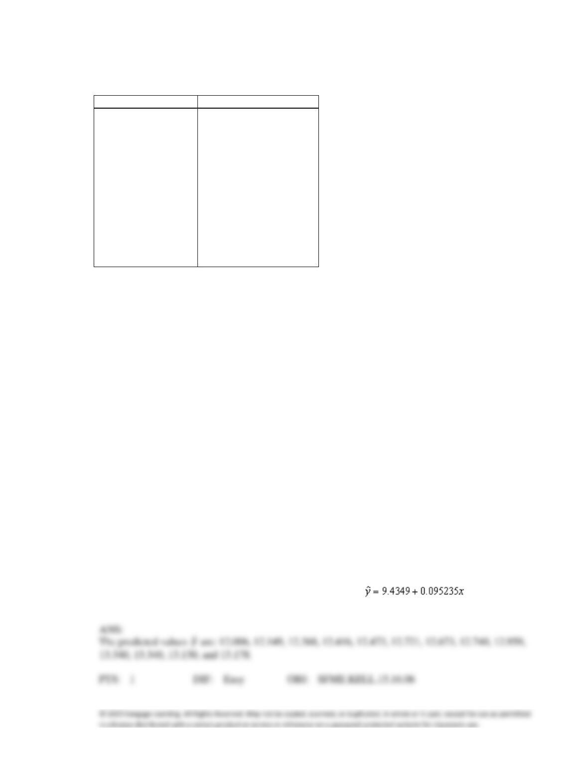
22. {Oil Quality and Price Narrative} Use the regression equation to determine
the predicted values of y.
23. {Oil Quality and Price Narrative} Use the predicted values and the actual values of y to calculate the
residuals.
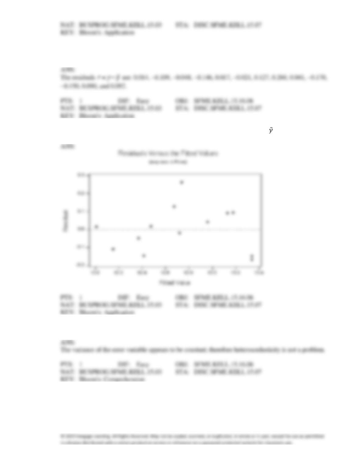
24. {Oil Quality and Price Narrative} Plot the residuals against the predicted values .
25. {Oil Quality and Price Narrative} Does it appear that heteroscedasticity is a problem? Explain.
26. {Oil Quality and Price Narrative} Draw a histogram of the residuals.
ANS:
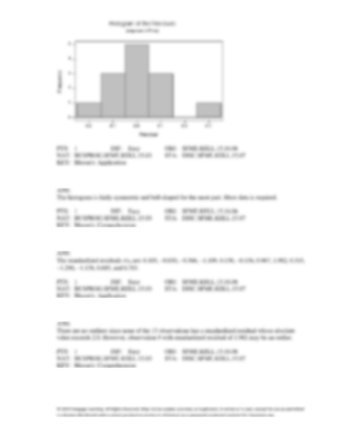
27. {Oil Quality and Price Narrative} Does it appear that the errors are normally distributed? Explain.
28. {Oil Quality and Price Narrative} Use the residuals to compute the standardized residuals.
29. {Oil Quality and Price Narrative} Identify possible outliers.