CHAPTER 16A: SIMPLE LINEAR REGRESSION AND CORRELATION
TRUE/FALSE
1. An inverse relationship between an independent variable x and a dependent variably y means that as x
increases, y decreases, and vice versa.
2. A direct relationship between an independent variable x and a dependent variably y means that the
variables x and y increase or decrease together.
3. Another name for the residual term in a regression equation is random error.
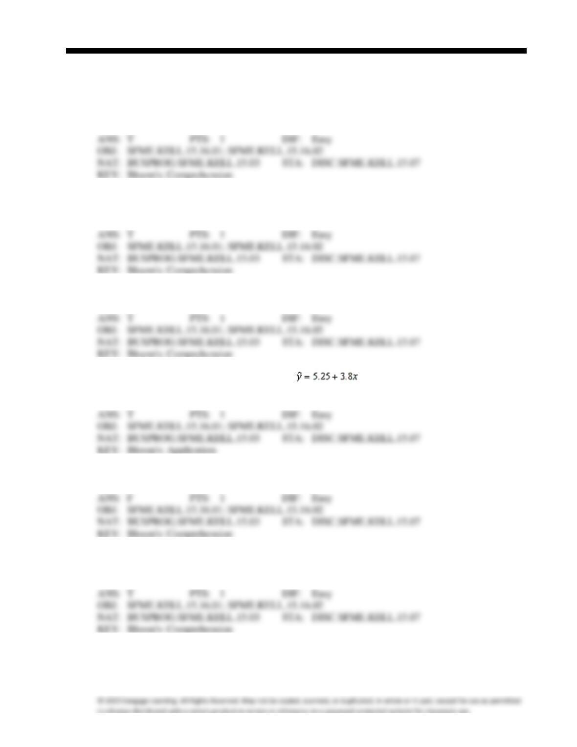
4. A simple linear regression equation is given by . The point estimate of y when x = 4 is
20.45.
5. The vertical spread of the data points about the regression line is measured by the y-intercept.
6. The method of least squares requires that the sum of the squared deviations between actual y values in
the scatter diagram and y values predicted by the regression line be minimized.
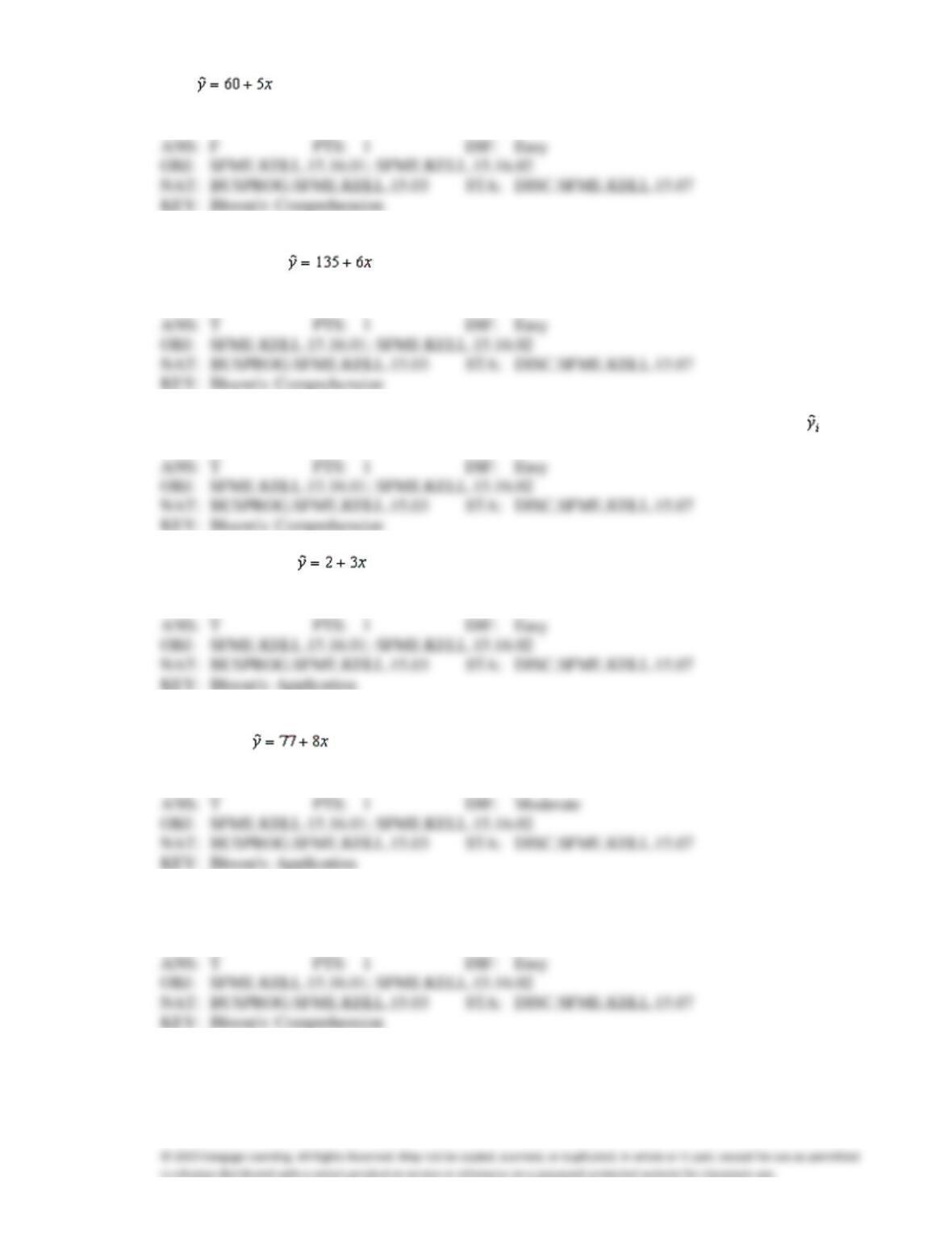
7. A regression analysis between sales (in $) and advertising (in $) resulted in the following least squares
line: . This implies that an increase of $1 in advertising is associated with an increase of
$60 in sales.
8. A regression analysis between weight (y in pounds) and height (x in inches) resulted in the following
least squares line: . This implies that if the height is increased by 1 inch, the weight is
expected to increase by an average of 6 pounds.
9. The residual ri is defined as the difference between the actual value yi and the estimated value .
10. The regression line has been fitted to the data points (4, 11), (2, 7), and (1, 5). The sum of
squares for error will be 10.0.
11. A regression analysis between sales (in $1000) and advertising (in $100) resulted in the following least
squares line: . This implies that if advertising is $600, then the predicted amount of sales
(in dollars) is $125,000.
12. The residuals are observations of the error variable
. Consequently, the minimized sum of squared
deviations is called the sum of squares for error, denoted SSE.
13. Statisticians have shown that sample y–intercept b0 and sample slope coefficient b1 are unbiased
estimators of the population regression parameters
0 and
1, respectively.
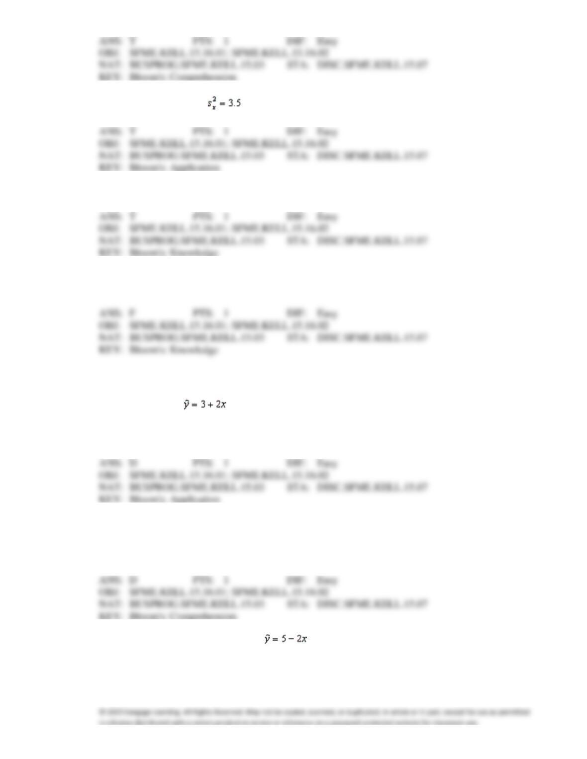
14. If cov(x, y) = 7.5075 and , then the sample slope coefficient is 2.145.
15. The first-order linear model is sometimes called the simple linear regression model.
16. To create a deterministic model, we start with a probabilistic model that approximates the relationship
we want to model.
MULTIPLE CHOICE
1. The regression line has been fitted to the data points (4, 8), (2, 5), and (1, 2). The sum of
the squared residuals will be:
a.
7
c.
8
b.
15
d.
22
2. If an estimated regression line has a y-intercept of 10 and a slope of 4, then when x = 2 the actual value
of y is:
a.
18
c.
14
b.
15
d.
unknown.
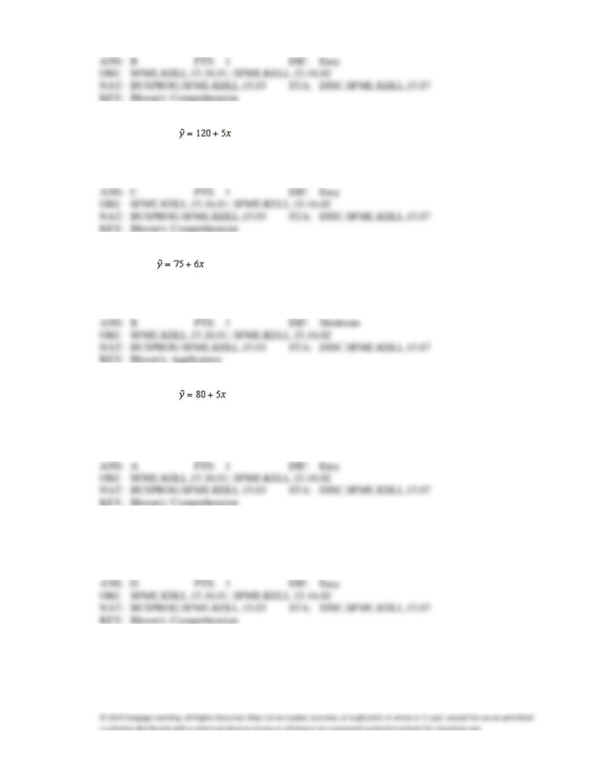
3. Given the least squares regression line :
a.
the relationship between x and y is positive.
b.
the relationship between x and y is negative.
c.
as x decreases, so does y.
d.
None of these choices.
4. A regression analysis between weight (y in pounds) and height (x in inches) resulted in the following
least squares line: . This implies that if the height is increased by 1 inch, the weight, on
average, is expected to:
a.
increase by 1 pound.
c.
increase by 5 pounds.
b.
decrease by 1 pound.
d.
increase by 24 pounds.
5. A regression analysis between sales (in $1000) and advertising (in $100) resulted in the following least
squares line: . This implies that if advertising is $800, then the predicted amount of sales
(in dollars) is:
a.
$4875
c.
$487,500
b.
$123,000
d.
$12,300
6. A regression analysis between sales (in $1,000) and advertising (in $1,000) resulted in the following
least squares line: . This implies that:
a.
as advertising increases by $1,000, sales increases by $5,000.
b.
as advertising increases by $1,000, sales increases by $80,000.
c.
as advertising increases by $5, sales increases by $80.
d.
None of these choices.
7. Which of the following techniques is used to predict the value of one variable on the basis of other
variables?
a.
Correlation analysis
c.
Covariance
b.
Coefficient of correlation
d.
Regression analysis
8. The residual is defined as the difference between:
a.
the actual value of y and the estimated value of y
b.
the actual value of x and the estimated value of x
c.
the actual value of y and the estimated value of x
d.
the actual value of x and the estimated value of y
9. In the simple linear regression model, the y-intercept represents the:
a.
change in y per unit change in x.
c.
value of y when x = 0.
b.
change in x per unit change in y.
d.
value of x when y = 0.
10. In the first order linear regression model, the population parameters of the y-intercept and the slope are
estimated, respectively, by:
a.
b0 and b1
c.
0 and b1
b.
b0 and
1
d.
0 and
1
11. In the simple linear regression model, the slope represents the:
a.
value of y when x = 0.
c.
value of x when y = 0.
b.
average change in y per unit change in x.
d.
average change in x per unit change in y.
12. In regression analysis, the residuals represent the:
a.
difference between the actual y values and their predicted values.
b.
difference between the actual x values and their predicted values.
c.
square root of the slope of the regression line.
d.
change in y per unit change in x.
13. In the first-order linear regression model, the population parameters of the y-intercept and the slope
are, respectively,
a.
b0 and b1
c.
0 and b1
b.
b0 and
1
d.
0 and
1
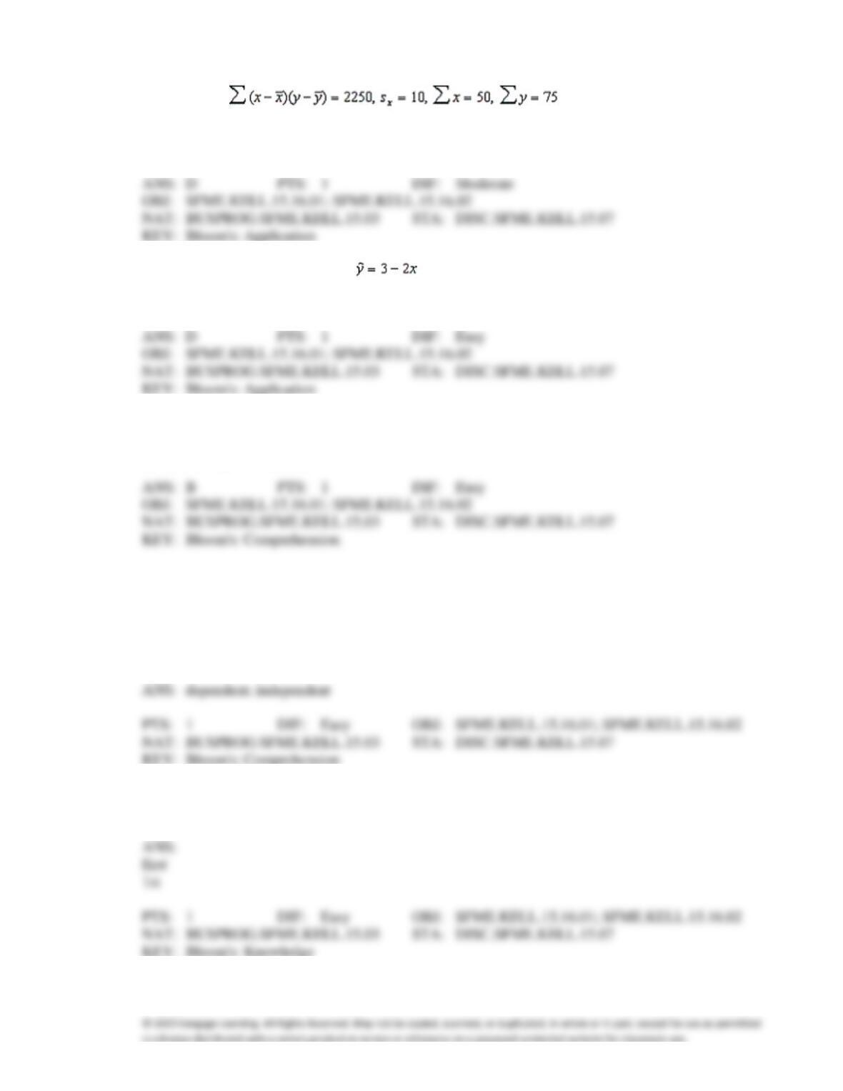
14. In a simple linear regression problem, the following statistics are calculated from a sample of 10
observations: . The least squares estimates of
the slope and y–intercept are, respectively,
a.
1.5 and 0.5
c.
1.5 and 2.5
b.
2.5 and 1.5
d.
2.5 and −5.0
15. In the least squares regression line , the predicted value of y equals:
a.
1.0 when x = −1.0
c.
2.0 when x = −1.0
b.
2.0 when x = 1.0
d.
1.0 when x = 1.0
16. The least squares method for determining the best fit minimizes:
a.
total variation in the dependent variable
c.
sum of squares for regression
b.
sum of squares for error
d.
All of these choices are true.
COMPLETION
1. In regression analysis, you predict the value of one variable on the basis of one or more other related
variables. The variable being predicted is called the ____________________ variable, and the related
variables used to make the prediction are called ____________________ variables.
2. A straight line regression model with only one independent variable is called a(n)
____________________-order linear model.
3. The objective of a regression model is to analyze the relationship between two variables, x and y, both
of which must be based on ____________________ data.
4. The deviations between the actual data points and the fitted values from the model are called
____________________.
5. SSE stands for ____________________ of squares for ____________________.
6. In a simple linear regression model b1 is the ____________________ of the straight line.
7. In a simple linear regression model b0 is the ____________________ of the straight line.
8. Suppose the slope of a simple linear regression line between hours studying and exam score is 5. That
means as ____________________ increases by one, ____________________ increases by 5.
9. You cannot interpret the ____________________ of the simple linear regression line unless the value
of x = 0 lies within the range of where data was collected.
10. The method statisticians use to produce a straight line that minimizes the SSE is called the
____________________ method.
SHORT ANSWER
Speed vs Gas Mileage
An economist wanted to analyze the relationship between the speed of a car (x) and its gas mileage (y).
As an experiment a car is operated at several different speeds and for each speed the gas mileage is
measured. These data are shown below.
Speed
25
35
45
50
60
65
70
Gas Mileage
40
39
37
33
30
27
25
1. {Car Speed and Gas Mileage Narrative} Determine the least squares regression line.
2. {Car Speed and Gas Mileage Narrative} Estimate the gas mileage of a car traveling 70 mph.
3. The following 10 observations of variables x and y were collected.
x
1
2
3
4
5
6
7
8
9
10
y
25
22
21
19
14
15
12
10
6
2
Find the least squares regression line, and the estimated value of y when x = 3.
4. A scatter diagram includes the following data points:
x
3
2
5
4
5
y
8
6
12
10
14
Two regression models are proposed: (1) , and (2) . Using the least squares
method, which of these regression models provides the better fit to the data? Why?
5. Consider the following data values of variables x and y.
x
2
4
6
8
10
13
y
7
11
17
21
27
36
a.
Determine the least squares regression line.
b.
Find the predicted value of y for x = 9.
c.
What does the value of the slope of the regression line tell you?
c.
If x increases by one unit, y on average will increase by 2.637.
Sunshine and Melanoma
A medical researcher wanted to examine the relationship between the amount of sunshine (x) in hours,
and incidence of melanoma, a type of skin cancer (y). As an experiment he found the number of
melanoma cases detected per 100,000 of population and the average daily sunshine in eight counties
around the country. These data are shown below.
Average Daily Sunshine
5
7
6
7
8
6
4
3
Melanoma per 100,000
7
11
9
12
15
10
7
5
6. {Sunshine and Melanoma Narrative} Determine the least squares regression line.
7. {Sunshine and Melanoma Narrative} Draw a scatter diagram of the data and plot the least squares
regression line on it.
8. {Sunshine and Melanoma Narrative} Estimate the number of skin cancer cases per 100,000 people
who live in a state that gets 6 hours of sunshine on average.
9. {Sunshine and Melanoma Narrative} What does the value of the slope of the regression line tell you?
10. {Sunshine and Melanoma Narrative} Calculate the residual corresponding to the pair (x, y) = (8, 15).
Sales and Experience
The general manager of a chain of department stores believes that experience is the most important
factor in determining the level of success of a salesperson. To examine this belief she records last
month’s sales (in $1,000s) and the years of experience of 10 randomly selected salespeople. These data
are listed below.
Salesperson
Years of Experience
Sales
1
0
7
2
2
9
3
10
20
4
3
15
5
8
18
6
5
14
7
12
20
8
7
17
9
20
30
10
15
25
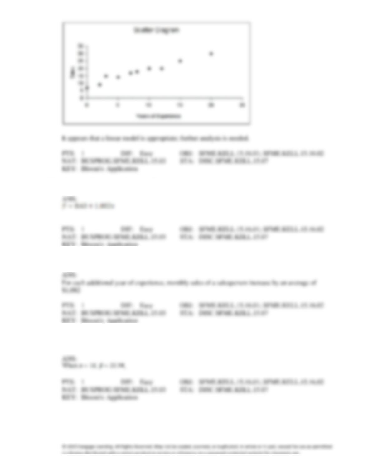
11. {Sales and Experience Narrative} Draw a scatter diagram of the data. Comment on whether it appears
that a linear model might be appropriate.
ANS:
12. {Sales and Experience Narrative} Determine the least squares regression line.
13. {Sales and Experience Narrative} Interpret the value of the slope of the regression line.
14. {Sales and Experience Narrative} Estimate the monthly sales for a salesperson with 16 years of
experience.
Income and Education
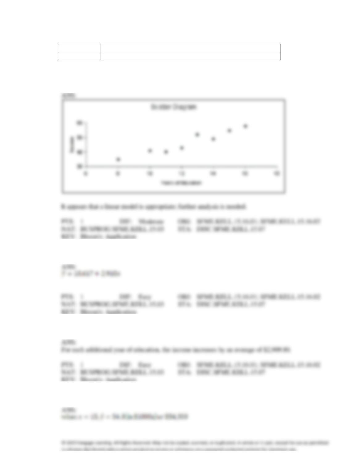
A professor of economics wants to study the relationship between income (y in $1000s) and education
(x in years). A random sample eight individuals is taken and the results are shown below.
Education
16
11
15
8
12
10
13
14
Income
58
40
55
35
43
41
52
49
15. {Income and Education Narrative} Draw a scatter diagram of the data. Comment on whether it appears
that a linear model might be appropriate.
16. {Income and Education Narrative} Determine the least squares regression line.
17. {Income and Education Narrative} Interpret the value of the slope of the regression line.
18. {Income and Education Narrative} Estimate the income of an individual with 15 years of education.
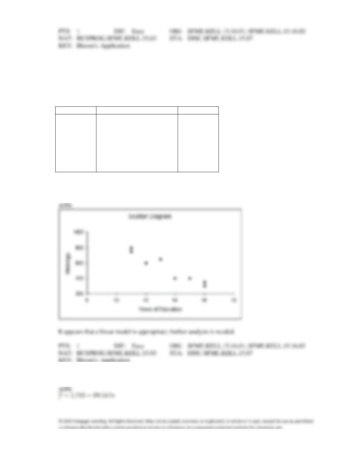
Trivia Games & Education
An ardent fan of television game shows has observed that, in general, the more educated the
contestant, the less money he or she wins. To test her belief she gathers data about the last eight
winners of her favorite game show. She records their winnings in dollars and the number of years of
education. The results are as follows.
Contestant
Years of Education
Winnings
1
11
750
2
15
400
3
12
600
4
16
350
5
11
800
6
16
300
7
13
650
8
14
400
19. {Trivia Games & Education Narrative} Draw a scatter diagram of the data. Comment on whether it
appears that a linear model might be appropriate.
20. {Trivia Games & Education Narrative} Determine the least squares regression line.
21. {Trivia Games & Education Narrative} Interpret the value of the slope of the regression line.
22. {Trivia Games & Education Narrative} Estimate the game winnings for a contestant with 15 years of
education.
Theatre Revenues
A financier whose specialty is investing in stage productions has observed that, in general, movies
with “big-name” stars seem to generate more revenue than those plays whose stars are less well
known. To examine his belief he records the gross revenue and the payment (in $ millions) given to
the two highest-paid performers in the play for ten recently staged plays.
Play
Cost of Two Highest Paid
Gross Revenue
Performers ($mil)
($mil)
1
5.3
48
2
7.2
65
3
1.3
18
4
1.8
20
5
3.5
31
6
2.6
26
7
8.0
73
8
2.4
23
9
4.5
39
10
6.7
58
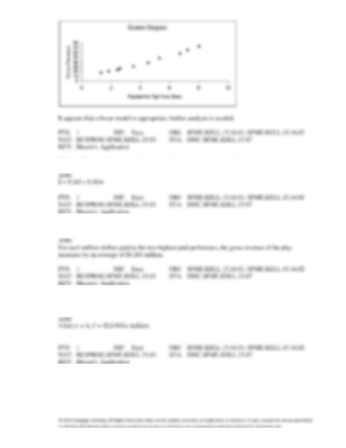
23. {Theatre Revenues Narrative} Draw a scatter diagram of the data. Comment on whether it appears that
a linear model might be appropriate.
ANS:
24. {Theatre Revenues Narrative} Determine the least squares regression line.
25. {Theatre Revenues Narrative} Interpret the value of the slope of the regression line.
26. {Theatre Revenues Narrative} Estimate the gross revenue of a play if the two highest paid performers
received 6 million dollars.
27. {Theatre Revenues Narrative} Are the two highest paid performers worth all the money paid for them?
Comment using the statistical analyses you have done.
ANS:
Cost of Textbooks
The editor of a higher education book publisher claims that a large part of the cost of books is the cost
of paper. This implies that larger textbooks will cost more money. As an experiment to analyze the
claim, a university student visits the bookstore and records the number of pages and the selling price of
twelve randomly selected textbooks. These data are listed below.
Textbook
Number of Pages
Selling Price ($)
1
844
55
2
727
50
3
360
35
4
915
60
5
295
30
6
706
50
7
410
40
8
905
53
9
1058
65
10
865
54
11
677
42
12
912
58
28. {Cost of Textbooks Narrative} Determine the least squares regression line.
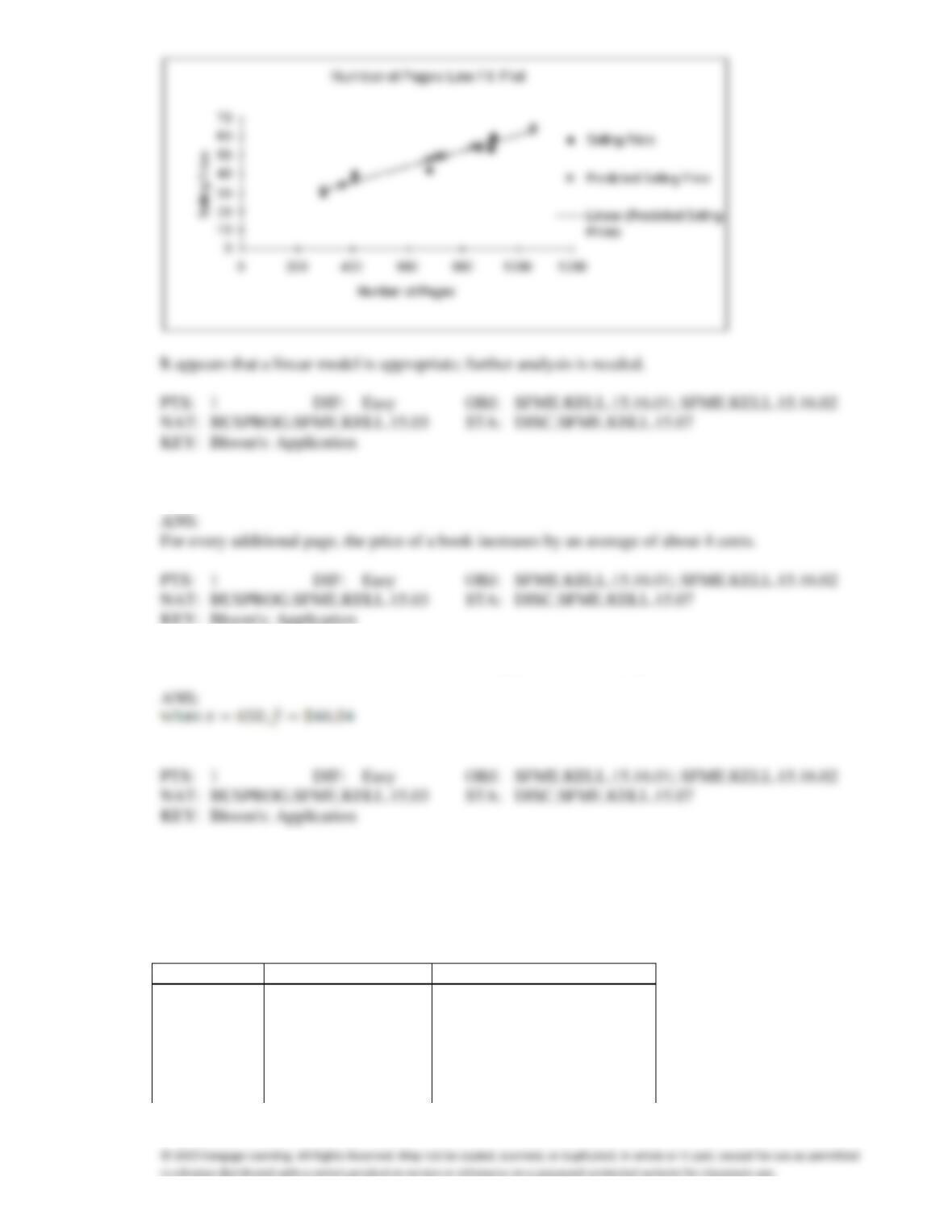
29. {Cost of Textbooks Narrative} Draw a scatter diagram of the data. Comment on whether it appears
that a linear model might be appropriate.
ANS:
30. {Cost of Textbooks Narrative} Interpret the value of the slope of the regression line.
31. {Cost of Textbooks Narrative} Estimate the selling price for a 650 pages book.
Accidents and Rain
A statistician investigating the relationship between the amount of rain (in inches) and the number of
automobile accidents gathered data on accidents in her city for 10 randomly selected days throughout
the year. The results are shown below.
Day
Rain
Number of Accidents
1
0.05
5
2
0.12
6
3
0.05
2
4
0.08
4
5
0.10
8
6
0.35
14
7
0.15
7
8
0.30
13
9
0.10
7
10
0.20
10
32. {Accidents and Rain Narrative} Find the least squares regression line.
33. {Accidents and Rain Narrative} Estimate the number of accidents in a day with 0.25 inches of rain.
34. {Accidents and Rain Narrative} What does the slope of the least squares regression line tell you?
35. {Accidents and Rain Narrative} What other variables might be associated with accidents, besides or
along with rain?
Allman Brothers Concert
At a recent Allman Brothers concert, a survey was conducted that asked a random sample of 20 people
their age and how many concerts they have attended since the first of the year. The following data
were collected:
Age
62
57
40
49
67
54
43
65
54
41
Number of Concerts
6
5
4
3
5
5
2
6
3
1
Age
44
48
55
60
59
63
69
40
38
52
Number of Concerts
3
2
4
5
4
5
4
2
1
3
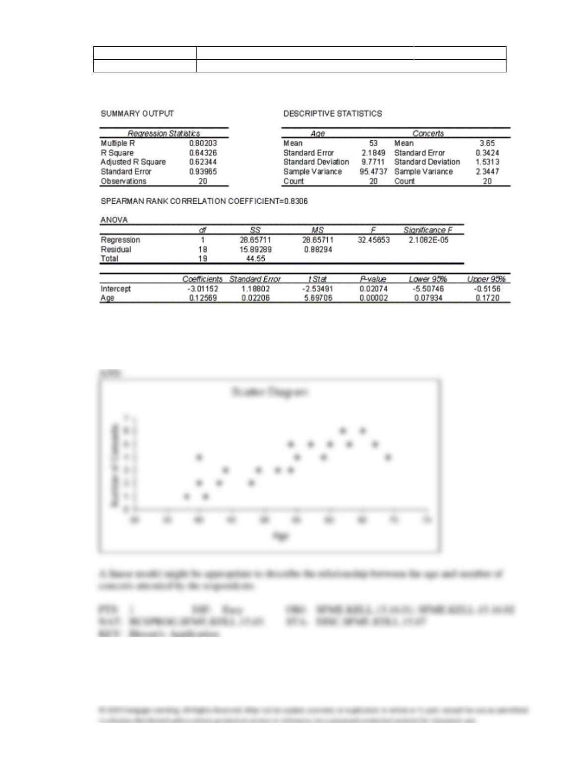
An Excel output follows:
36. {Allman Brothers Concert Narrative} Draw a scatter diagram of the data. Comment on whether it
appears that a linear model might be appropriate to describe the relationship between the age and
number of concerts attended by the respondents.
37. {Allman Brothers Concert Narrative} Determine the least squares regression line.