CHAPTER 13: INFERENCE ABOUT COMPARING TWO POPULATIONS
TRUE/FALSE
1. Independent samples are those for which the selection process for one is not related to the selection
process for the other.
2. In testing the difference between two population means using two independent samples, the sampling
distribution of the sample mean difference is normal if the sample sizes are both greater than
30.
3. The pooled-variances t-test requires that the two population variances need not be the same.
4. In testing the difference between two population means using two independent samples, we use the
pooled variance in estimating the standard error of the sampling distribution of the sample mean
difference if the populations are normal with equal variances.
5. A political analyst in Iowa surveys a random sample of registered Republicans and compares the
results with those obtained from a random sample of registered Democrats . This would be an example
of two independent samples.
6. Two samples of sizes 25 and 20 are independently drawn from two normal populations, where the
unknown population variances are assumed to be equal. The number of degrees of freedom of the
equal-variances t-test statistic is 44.
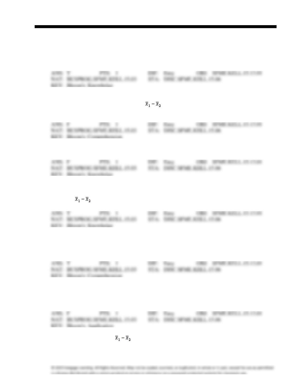
7. The sampling distribution of is normal if the sampled populations are normal, and
approximately normal if the populations are nonnormal and the sample sizes n1 and n2 are large.
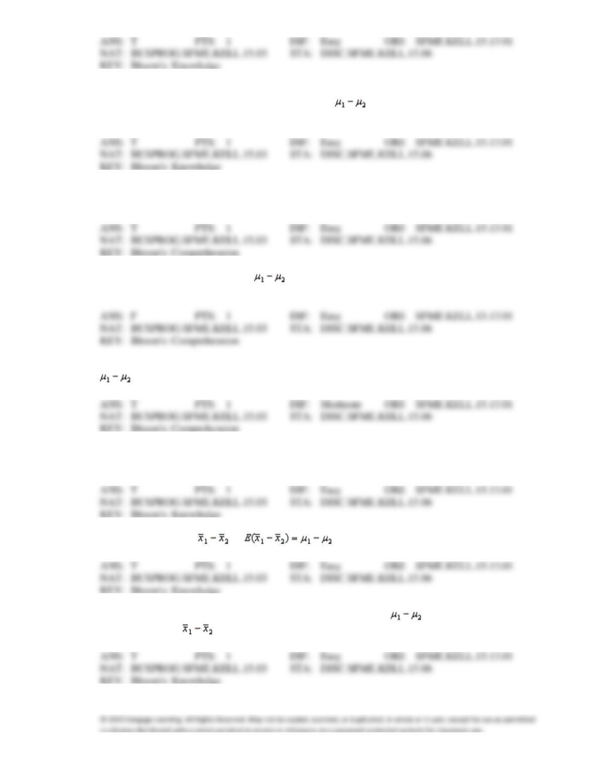
8. When the population variances are unequal, we estimate each population variance with its sample
variance. Hence, the unequal-variances test statistic of is approximately Student t–distributed
with n1 + n2 − 2 degrees of freedom.
9. Unless we can conclude that the population variances are equal, we cannot use the pooled variance
estimate.
10. The equal-variances test statistic of is Student t-distributed with n1 + n2 degrees of freedom,
provided that the two populations are normal.
11. Both the equal-variances and unequal variances test statistic and confidence interval estimator of
require that the two populations be normally distributed.
12. When the sample sizes are equal, the pooled variance of the two samples is the weighted average of
the two sample variances.
13. The expected value of is .
14. The best estimator of the difference between two population means is the difference between
two sample means .
15. When we test for differences between the means of two independent populations, we can only use a
two-tailed test.
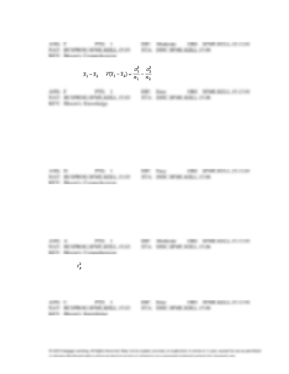
16. The variance of is .
MULTIPLE CHOICE
1. The expected value of the difference of two sample means equals the difference of the corresponding
population means when:
a.
the populations are normally distributed.
b.
the samples are independent.
c.
the populations are approximately normal and the sample sizes are large.
d.
All of these choices are true.
2. In testing the difference between the means of two normally distributed populations, the number of
degrees of freedom associated with the unequal-variances t-test statistic usually results in a non-integer
number. It is recommended that you:
a.
round to the nearest integer.
b.
change the sample sizes until the number of degrees of freedom becomes an integer.
c.
assume that the population variances are equal, and then use df = n1 + n2 − 2.
d.
None of these choices.
3. The quantity is called the pooled variance estimate of the common variance of two unknown but
equal population variances. It is the weighted average of the two sample variances, where the weights
represent the:
a.
sample variances.
c.
degrees of freedom for each sample.
b.
sample standard deviations.
d.
None of these choices.
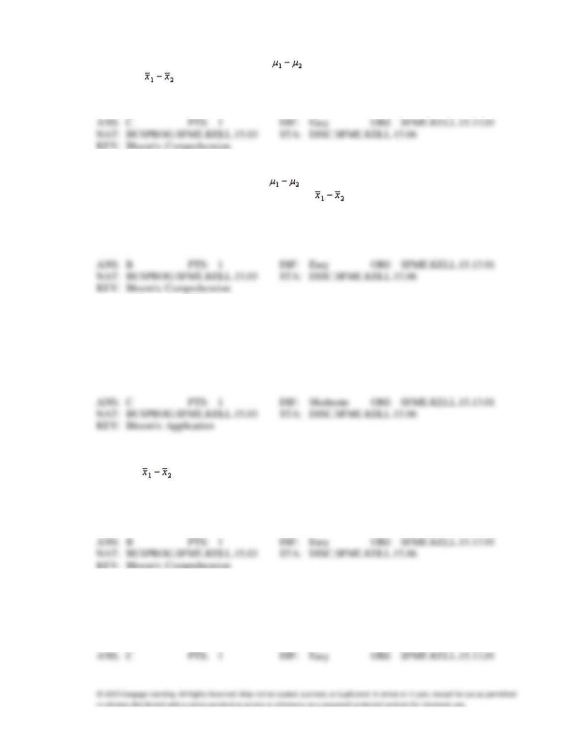
4. Two independent samples of sizes 20 and 30 are randomly selected from two normally distributed
populations. Assume that the population variances are unknown but equal. In order to test the
difference between the population means, , the sampling distribution of the sample mean
difference, , is:
a.
normal.
c.
Student-t with 48 degrees of freedom.
b.
Student-t with 50 degrees of freedom.
d.
None of these choices.
5. Two independent samples of sizes 40 and 50 are randomly selected from two populations to test the
difference between the population means . Assume the population variances are known. The
sampling distribution of the sample mean difference is:
a.
normally distributed.
b.
approximately normal.
c.
Student t-distributed with 88 degrees of freedom.
d.
None of these choices.
6. Two independent samples of sizes 25 and 35 are randomly selected from two normal populations with
equal variances (assumed to be unknown). In order to test the difference between the population
means, the test statistic is:
a.
a standard normal random variable.
b.
approximately standard normal random variable.
c.
Student t-distributed with 58 degrees of freedom.
d.
Student t-distributed with 33 degrees of freedom.
7. In testing the difference between two population means using two independent samples, we use the
pooled variance in estimating the standard error of the sampling distribution of the sample mean
difference if:
a.
the sample sizes are both large.
b.
the populations are normal with equal variances.
c.
the populations are non-normal with unequal variances.
d.
All of these choices are true.
8. In testing the difference between two population means for which the population variances are
unknown and not assumed to be equal, two independent samples are drawn from the populations.
Which of the following tests is appropriate?
a.
z-test
c.
unequal variances t–test
b.
pooled-variances t-test
d.
None of these choices.
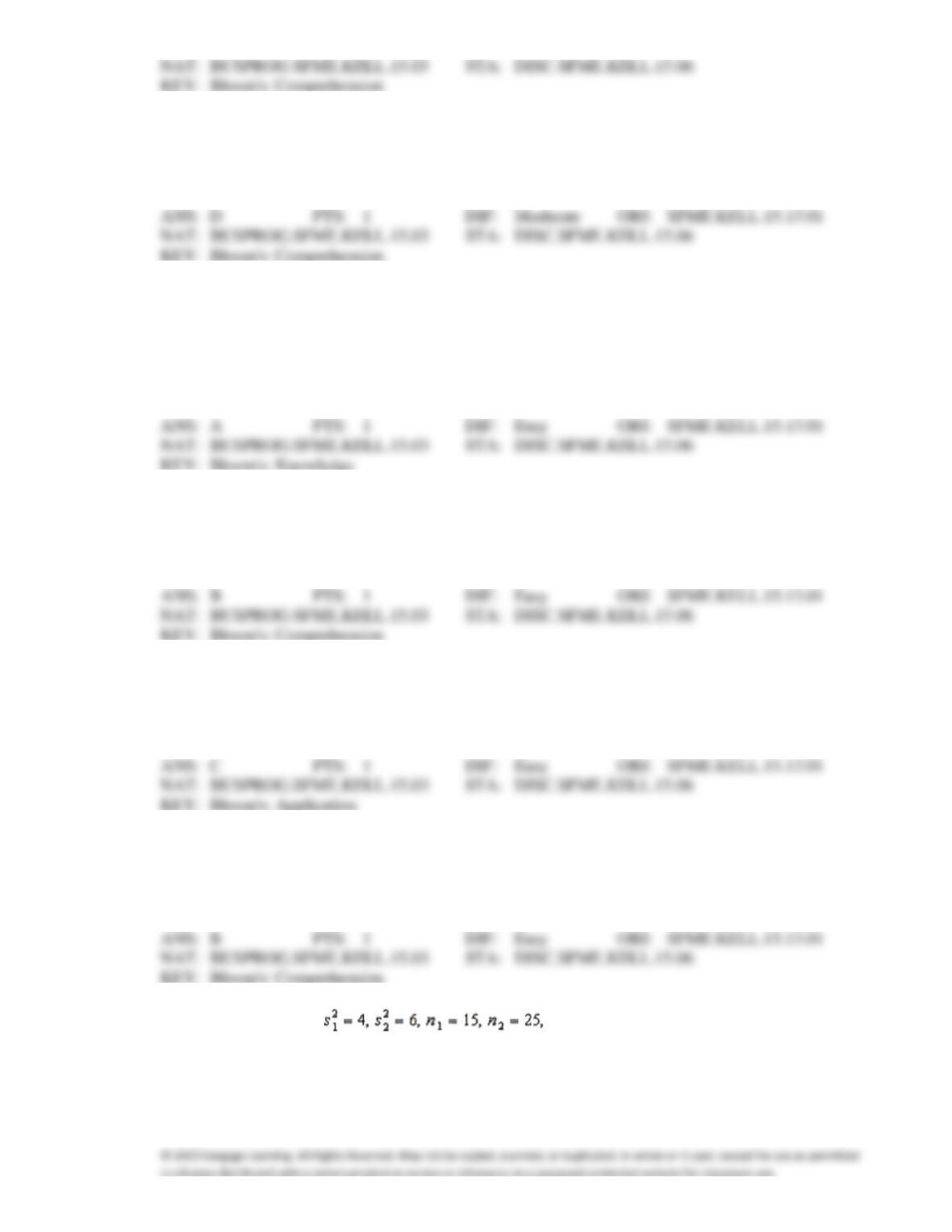
9. In testing the difference between the means of two normal populations using two independent samples
when the population variances are unequal, the sampling distribution of the resulting statistic is:
a.
normal.
c.
approximately normal.
b.
Student-t.
d.
approximately Student-t.
10. In constructing a confidence interval estimate for the difference between the means of two independent
normally distributed populations, we:
a.
pool the sample variances when the unknown population variances are equal.
b.
pool the sample variances when the population variances are known and equal.
c.
pool the sample variances when the population means are equal.
d.
never pool the sample variances.
11. The t–test for the difference between the means of two independent populations assumes that the
respective:
a.
sample sizes are equal.
c.
means are equal.
b.
populations are normal.
d.
All of these choices are true.
12. If we are testing for the difference between the means of two independent populations with equal
variances, samples of n1 = 15 and n2 = 15 are taken, then the number of degrees of freedom is equal to
a.
13
c.
28
b.
14
d.
29
13. In testing for the differences between the means of two independent populations where the variances in
each population are unknown but assumed equal, the degrees of freedom is:
a.
n1 + n2
c.
n1 + n2 − 1
b.
n1 + n2 − 2
d.
None of these choices
14. Given the information: the number of degrees of freedom that should
be used in the pooled variance t-test is:
a.
40
c.
15
b.
38
d.
25
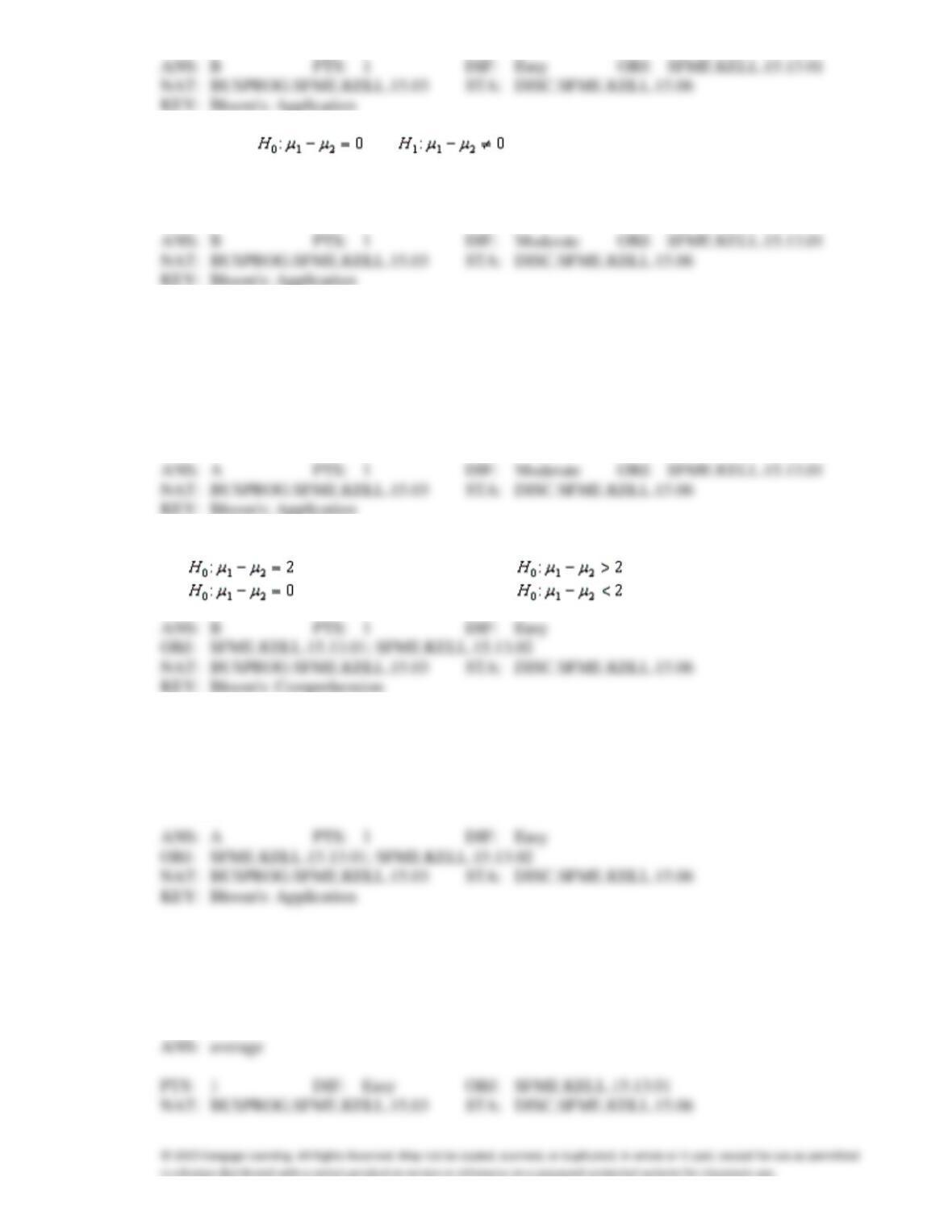
15. When testing vs. , the observed value of the z-score was found to be
−2.15. Then, the p–value for this test would be
a.
.0158
c.
.9842
b.
.0316
d.
.9684
16. A political analyst in Hawaii surveys a random sample of registered Democrats and compares the
results with those obtained from a random sample of registered Republicans. This would be an
example of:
a.
independent samples.
b.
dependent samples.
c.
independent samples only if the sample sizes are equal.
d.
dependent samples only if the sample sizes are equal.
17. In testing for differences between the means of two independent populations the null hypothesis is:
a.
c.
b.
d.
18. Suppose we randomly selected 250 people, and on the basis of their responses to a survey we assigned
them to one of two groups: high-risk group and low-risk group. We then recorded the blood pressure
for the members of each group. Such data are called:
a.
observational.
c.
matched.
b.
experimental.
d.
None of these choices.
COMPLETION
1. When the sample sizes are equal, the pooled variance of the two samples is the
____________________ of the two sample variances.
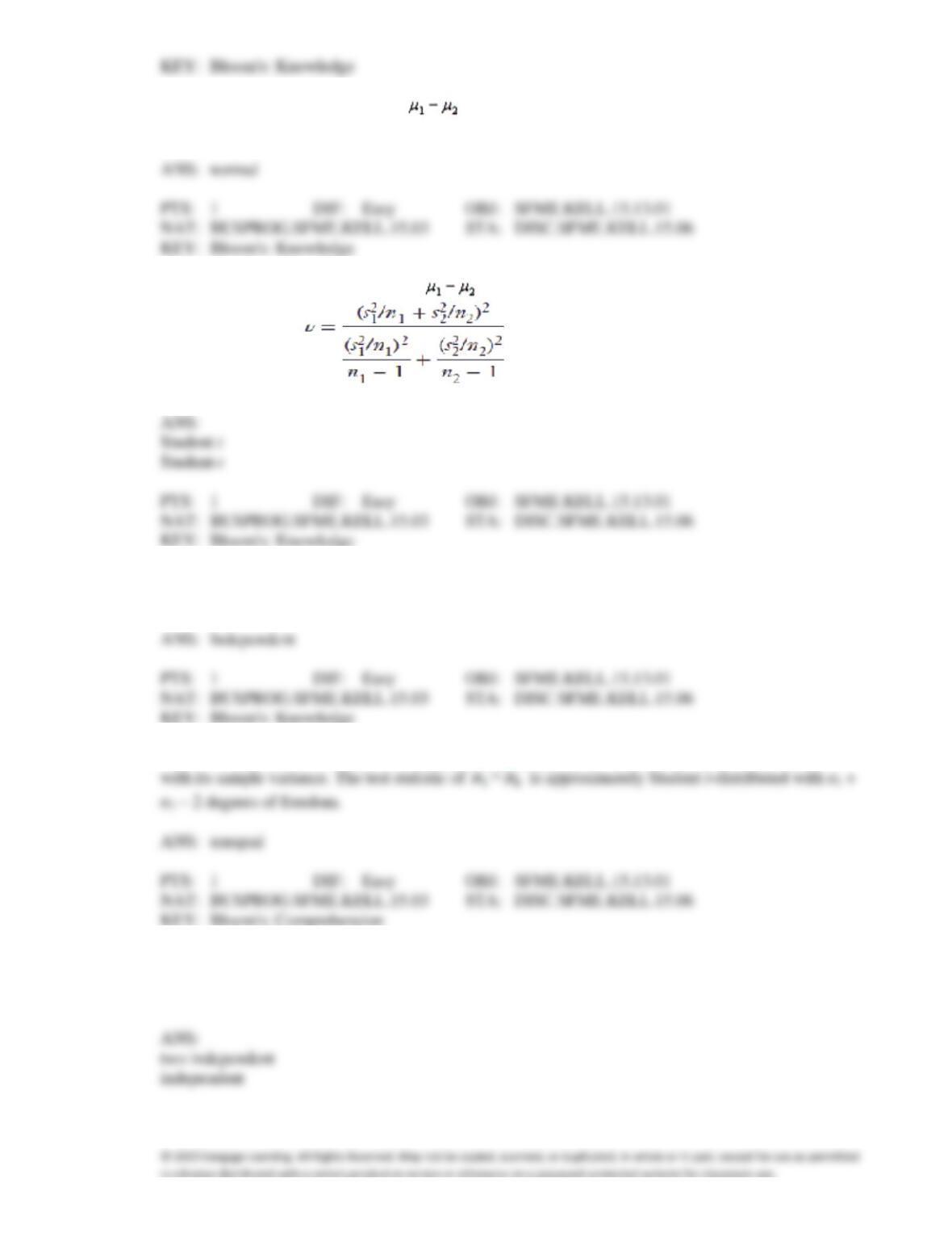
2. The equal-variances test statistic of is Student t-distributed with n1 + n2 − 2 degrees of
freedom provided that the two populations are ____________________.
3. The unequal-variances test statistic of has an approximate ____________________
distribution with degrees of freedom.
4. ____________________ samples are those for which the selection process for one is not related to the
selection process for the other.
5. When two population variances are ____________________ we estimate each population variance
6. A political analyst in Iowa surveys a random sample of registered Democrats and compares the results
with those obtained from a random sample of registered Republicans. This would be an example of
____________________ samples.
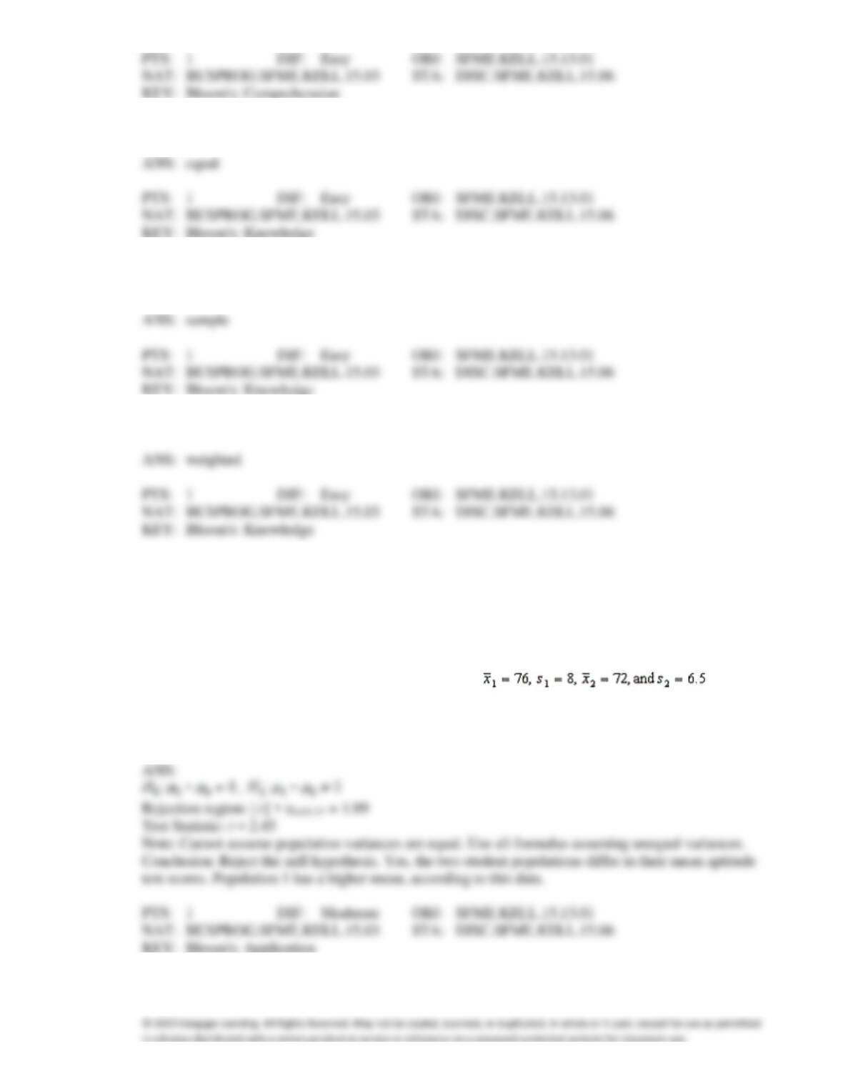
7. The pooled-variances t-test is used when the two population variances are ____________________.
8. When the population variances are unknown and unequal, we estimate each population variance with
its ____________________ variance.
9. The pooled variance estimator is the ____________________ average of the two sample variances.
SHORT ANSWER
Aptitude Test Scores
Two random samples of 40 students were drawn independently from two populations of students.
Assume their aptitude tests are normally distributed (total points = 100). The following statistics
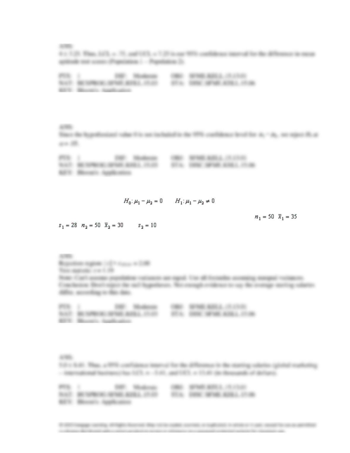
regarding their scores in an aptitude test were obtained: .
1. {Aptitude Test Scores Narrative} Test at the 5% significance level to determine whether we can infer
that the two population means differ.
2. {Aptitude Test Scores Narrative} Estimate with 95% confidence the difference between the two
population means.
3. {Aptitude Test Scores Narrative} Explain how to use the 95% confidence interval to test the
hypotheses at
= .05.
Starting Salary
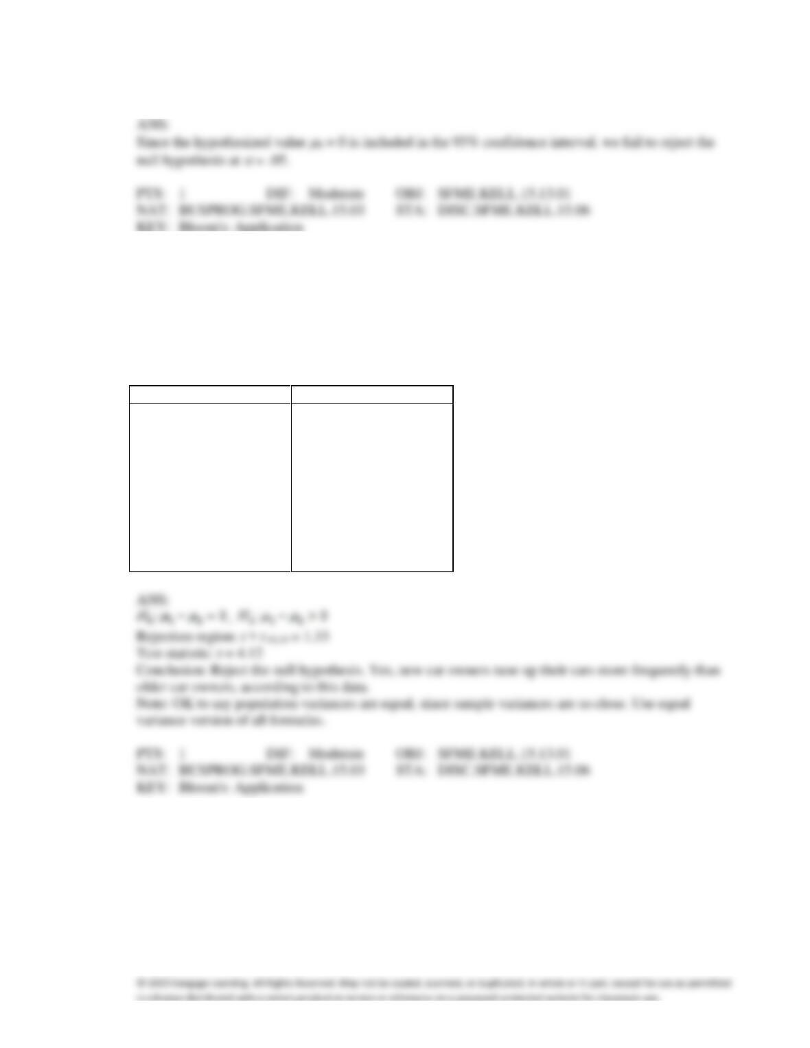
In testing the hypotheses vs. , two random samples from two
populations of college of business graduates majoring in global marketing and international business
produced the following statistics regarding their starting salaries (in $1000s): , ,
, , , and . (Assume the salaries have normal distributions.)
4. {Starting Salary Narrative} What conclusion can we draw at the 5% significance level?
5. {Starting Salary Narrative} Estimate with 95% confidence the difference between the two population
means.
6. {Starting Salary Narrative} Explain how to use the 95% confidence interval to test the hypotheses at
= .05.
7. The service manager of a car dealer wants to determine if owners of new cars (two years old or less)
tune up their cars more frequently than owners of older cars (more than two years old). From his
records he takes a random sample of ten new cars and ten older cars and determines the number of
times the cars were tuned up in the last 12 months. The data follow. Do these data allow the service
station owner to infer at the 10% significance level that new car owners tune up their cars more
frequently than older car owners?
Frequency of Tune Ups in Past 12 Months
New Car Owners
Old Cars Owners
6
4
3
2
3
1
3
2
4
3
3
2
6
2
5
3
5
2
4
1
Undergraduates’ Test Scores
35 undergraduate students who completed two years of college were asked to take a basic mathematics
test. The mean and standard deviation of their scores were 75.1 and 12.8, respectively. In a random
sample of 50 students who only completed high school, the mean and standard deviation of the test
scores were 72.1 and 14.6, respectively.
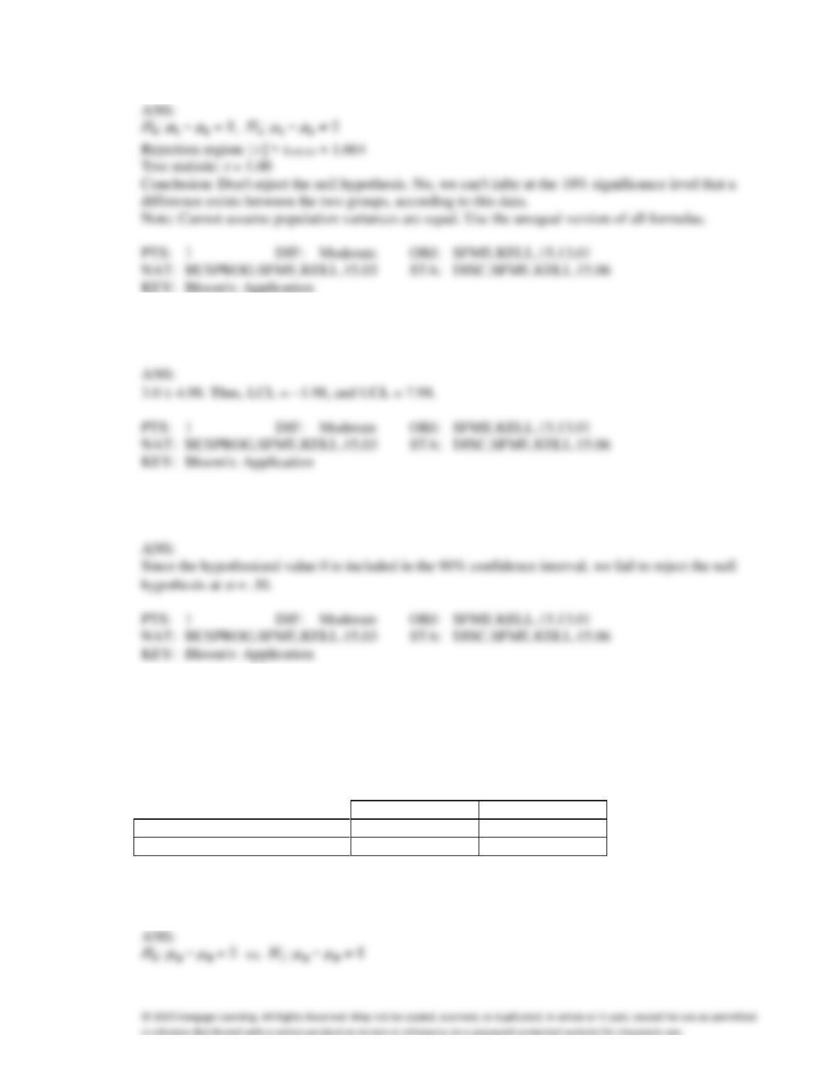
8. {Undergraduates’ Test Scores Narrative} Can we infer at the 10% significance level that a difference
exists between the two groups?
9. {Undergraduates’ Test Scores Narrative} Estimate with 90% confidence the difference in mean scores
between the two groups of students.
10. {Undergraduates’ Test Scores Narrative} Explain how to use the interval estimate to test the
hypotheses.
Additives
A food processor wants to compare two additives for their effects on retarding spoilage. Suppose 16
cuts of fresh meat are treated with additive A and 16 are treated with additive B, and the number of
hours until spoilage begins is recorded for each of the 32 cuts of meat. The results are summarized in
the table below
Additive A
Additive B
Sample Mean
108.7 hours
98.7 hours
Sample Standard Deviation
10.5 hours
13.6 hours
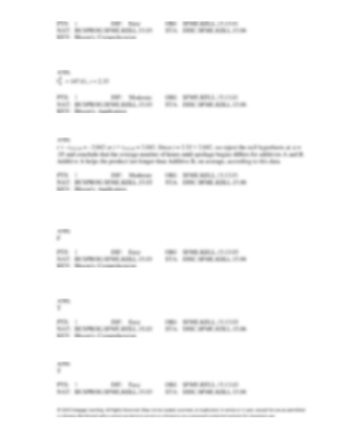
11. {Additives Narrative} State the null and alternative hypotheses to determine if the average number of
hours until spoilage begins differs for the additives A and B.
12. {Additives Narrative} Assume population variances are equal. Calculate the pooled variance and the
value of the test statistic.
13. {Additives Narrative} Determine the rejection region at
= .05 and write the proper conclusion.
14. A calculus professor wanted to test whether the grades on calculus test were the same for upper and
lower classmen. The professor took a random sample of size 12 from each group. For this situation,
the professor should use a matched pairs t-test.
15. Two measurements from the same individuals is an example of data collected from a matched pairs
experiment.
16. A matched pairs experiment decreases variability (compared to two independent samples).
17. In comparing the difference in means with a matched pairs experiment, the variable under
consideration is , where the subscript D refers to the difference.
18. The number of degrees of freedom associated with the t-test, when the data are gathered from a
matched pairs experiment with 8 pairs, is 7.
19. When comparing two population means using data that are gathered from a matched pairs experiment,
the test statistic for
D is Student t-distributed with v = nD − 1 degrees of freedom, provided that the
differences are normally distributed.
20. In comparing two population means of interval data, we must decide whether the samples are
independent (in which case the parameter of interest is ) or matched pairs (in which case the
parameter is
D) in order to select the correct test statistic.
21. If there are 10 pairs of data in a matched pairs experiment, the degrees of freedom for the
corresponding t-test is 18.
22. A Marine boot camp instructor recorded the time in which each of 15 recruits completed an obstacle
course both before and after basic training. To test whether any improvement occurred, the instructor
would use a t–distribution with 15 degrees of freedom.
23. A test is being conducted to test the difference between two population means using data that are
gathered from a matched pairs experiment. If the paired differences are normal, then the distribution
used for testing is the:
a.
normal distribution.
b.
binomial distribution.
c.
Student t-distribution.
d.
F-distribution.
24. If some natural relationship exists between each pair of observations that provides a logical reason to
compare the first observation of sample 1 with the first observation of sample 2, the second
observation of sample 1 with the second observation of sample 2, and so on, the samples are referred
to as:
a.
matched pairs.
b.
independent samples.
c.
nonrandom samples.
d.
None of these choices.
25. The number of degrees of freedom associated with the t-test, when the data are gathered from a
matched pairs experiment with 10 pairs, is:
a.
10
b.
20
c.
9
d.
18
26. The symbol refers to:
a.
the difference in the means of two independent populations.
b.
one matched pairs difference.
c.
the mean difference in the pairs of observations.
d.
None of these choices.
27. In testing for a mean difference the null hypothesis is:
a.
b.
c.
d.
None of these choices.
28. Two measurements from the same individuals is an example of data collected from a(n)
____________________ experiment.
29. The test for the mean difference in a matched pairs design requires the differences to have a(n)
____________________ distribution.
30. The degrees of freedom for a test of the mean of the paired differences is the number of
____________________ minus ____________________.
31. In a matched pairs experiment the parameter of interest is the ____________________ of the
population of ____________________.
32. If you are testing to see if a weight loss program is working, and you subtract the weights before −
after for a group of 10 people, the alternative hypothesis is that the mean difference is
____________________ 0.
33. If you are testing to see if a weight loss program is working, and you subtract the weights after −
before for a group of 10 people, the alternative hypothesis is that the mean difference is
____________________ 0.
34. In testing the hypothesis vs. , two random samples from two normal
populations produced the following statistics: . What conclusion can we
draw at the 1% significance level?
Engine Wear
To compare the wearing of two types of automobile engines, 1 and 2, an experimenter chose to “pair”
the measurements, comparing the wear for the two types of engines on each of 7 automobiles, as
shown below.
Automobile
1
2
3
4
5
6
7
Engine 1
8
15
7
9
10
13
11
Engine 2
12
18
8
9
12
11
10
35. (Engine Wear Narrative} Determine whether these data are sufficient to infer at the 10% significance
level that the two types of engines wear differently.
36. {Engine Wear Narrative} Estimate with 90% confidence the mean difference and interpret.
Promotional Campaigns
The general manager of a chain of fast food chicken restaurants wants to determine how effective their
promotional campaigns are. In these campaigns “20% off” coupons are widely distributed. These
coupons are only valid for one week. To examine their effectiveness, the executive records the daily
gross sales (in $1,000s) in one restaurant during the campaign and during the week after the campaign
ends. The data is shown below.
Day
Sales During Campaign
Sales After Campaign
Sunday
18.1
16.6
Monday
10.0
8.8
Tuesday
9.1
8.6
Wednesday
8.4
8.3
Thursday
10.8
10.1
Friday
13.1
12.3
Saturday
20.8
18.9
37. {Promotional Campaigns Narrative} Can they infer at the 5% significance level that sales increase
during the campaign?
38. {Promotional Campaigns Narrative} Estimate with 95% confidence the mean difference and interpret.
39. Motorcycle insurance appraisers examine motorcycles that have been involved in accidental collisions
to assess the cost of repairs. An insurance executive is concerned that different appraisers produce
significantly different assessments. In an experiment 10 motorcycles that have recently been involved
in accidents were shown to two appraisers. Each assessed the estimated repair costs. These results are
shown below. Can the executive conclude at the 5% significance level that the appraisers differ in their
assessments?
Motorcycle
Appraiser 1
Appraiser 2
1
1650
1400
2
360
380
3
640
600
4
1010
920
5
890
930
6
750
650
7
440
410
8
1210
1080
9
520
480
10
690
770
Clothing Expenditures
A marketing consultant was in the process of studying the perceptions of married couples concerning
their monthly clothing expenditures. He believed that the husband’s perception would be higher than
the wife’s. To judge his belief, he takes a random sample of ten married couples and asks each spouse
to estimate the family clothing expenditure (in dollars) during the previous month. The data are shown
below.
Couple
Husband
Wife
1
380
270
2
280
300
3
215
185
4
350
320
5
210
180
6
410
390
7
250
250
8
360
320
9
180
170
10
400
330
40. {Clothing Expenditures Narrative} Can the consultant conclude at the 5% significance level that the
husband’s estimate is higher than the wife’s estimate?
41. {Clothing Expenditures Narrative} Estimate with 95% confidence the population mean difference.
42. {Clothing Expenditures Narrative} Briefly describe what the interval estimate tells you.
43. A behaviorist has performed the following experiment. For each of 10 sets of identical twins who were
born 30 years ago, he recorded their annual incomes, according to which twin was born first. The
results (in $1,000s) are shown below. Can he infer at 5% significance level that there is a difference in
income between the twins?
Twin Set
First Born
Second Born
1
32
44
2
36
43
3
21
28
4
30
39
5
49
51
6
27
25
7
39
32
8
38
42
9
56
64
10
44
44
44. When comparing two population variances, we use the ratio rather than the difference
.
45. We use a t-test to determine whether two population variances are equal.