41. Demand Curve Analysis. Papa’s Pizza, Ltd., provides delivery and carryout service to the city of South
Bend, Indiana. An analysis of the daily demand for pizzas has revealed the following demand relation:
Q = 1,400 – 100P – 2PS + 0.01CSP + 750S
where Q is the quantity measured by the number of pizzas per day, P is the price ($), PS is a price index for soda pop (1992 = 100), CSP is the college
student population and S, a binary or dummy variable, equals 1 on Friday, Saturday and Sunday, zero otherwise.
A.
Determine the demand curve facing Papa’s Pizza on Tuesdays if P = $10, PS = 125, and CSP = 35,000, and S = 0.
B.
Calculate the quantity demanded and total revenues on Fridays if all price-related variables are as specified above.
Q
= 1,750 – 40P – 15PC + 30BAI – 1,700S
= 1,750 – 40P – 15(120) + 30(175) – 1,700(0)
Q
= 5,200 – 40P
Q
= 5,200 – 40P
= 5,200 – Q
P
= $130 – $0.025Q
Q
= 1,750 – 40(40) – 15(120) + 30(175) – 1,700(1)
= 1,900 passengers
= PQ
= $40(1,900)
= $76,000
42. Supply Curve Analysis. A review of industry-wide data for the domestic wine manufacturing industry
suggests the following industry supply function:
Q
= -7,000,000 + 400,000P – 2,000,000PL – 1,500,000P K + 1,000,000W
where Q is cases supplied per year, P is the wholesale price per case ($), PL is the average price paid for unskilled labor ($), PK is the average price of
capital (in percent), and W is weather measured by the average seasonal rainfall in growing areas (in inches).
A.
Determine the industry supply curve for a recent year when P = $80, PL = $10, PK = 12%, and W = 25 inches of rainfall. Show the
industry supply curve with quantity expressed as a function of price and price expressed as a function of quantity.
B.
Calculate the quantity supplied by the industry at prices of $50, $75 and $100 per case.
C.
Calculate the prices necessary to generate a supply of 10 million, 25 million, and 50 million cases.
With quantity expressed as a function of price, the industry supply curve can be written:
Q
= 1,400 – 100P – 2PS + 0.01CSP + 750S
= 1,400 – 100P – 2(125) + 0.01(35,000) + 750(0)
Q
= 1,500 – 100P
Q
= 1,500 – 100P
100P
= 1,500 – Q
P
= $15 – $0.01Q
B.
On Fridays, the variable S = 1. Therefore, assuming that price-related values remain as before, the quantity demanded on Fridays is:
Q
= 1,400 – 100(10) – 2(125) + 0.01(35,000) + 750(1)
= 1,250 pizzas.
Total revenue on Fridays
for the firm is:
= PQ
= $10(1,250)
= $12,500
43. Supply Curve Analysis. A review of industry-wide data for the frozen grape juice manufacturing industry
suggests the following industry supply function:
Q
= -3,000,000 + 500,000P – 800,000PL – 1,000,000PK + 300,000W
where Q is cases supplied per year, P is the wholesale price per case ($), PL is the average price paid for unskilled labor ($), PK is the average price of
capital (in percent), and W is weather measured by the average seasonal temperature in growing areas (in Fahrenheit).
A.
Determine the industry supply curve for a recent year when P = $40, PL = $10, PK = 15%, and W = 70 degrees Fahrenheit. Show the
industry supply curve with quantity expressed as a function of price and price expressed as a function of quantity.
B.
Calculate the quantity supplied by the industry at prices of $30, $40 and $50 per case.
C.
Calculate the prices necessary to generate a supply of 10 million, 25 million, and 40 million cases.
Q
= -7,000,000 + 400,000P – 2,000,000PL – 1,500,000PK + 1,000,000W
= -7,000,000 + 400,000P – 2,000,000(10) – 1,500,000(12)
+ 1,000,000(25)
can be written:
Q
= -20,000,000 + 400,000P
400,000P
= 20,000,000 + Q
P
= $50 + $0.0000025Q
B.
Industry supply at each respective price is:
P = $50:
Q
= -20,000,000 + 400,000(50) = 0
P = $75:
Q
= -20,000,000 + 400,000(75) = 10,000,000
P = $100:
Q
= -20,000,000 + 400,000(100) = 20,000,000
C.
The price necessary to generate each level of supply is:
Q = 10,000,000:
P
= $50 + $0.0000025(10,000,000) = $75
Q = 50,000,000:
P
= $50 + $0.0000025(50,000,000) = $175
44. Supply Curve Analysis. Computers.com is a leading Internet retailer of high-performance desktop
computers. Based on an analysis of monthly cost and output data, the company has estimated the following
relation between its marginal cost of production and monthly output:
MC = ¶ TC/ ¶ Q = $100 + $0.005Q
A.
Calculate the marginal cost of production at 100,000, 200,000, and 300,000 units of output.
B.
Express output as a function of marginal cost. Calculate the level of output at which MC = $1,000, $1,500 and $2,000.
C.
Calculate the profit-maximizing level of output if prices are stable in the industry at $1,500 per unit and, therefore, P = MR = $1,500.
D.
Again assuming prices are stable in the industry, derive the firm’s supply curve. Express price as a function of quantity and quantity as a
function of price.
Q
+ 300,000(70)
can be written:
Q
500,000P
= 5,000,000 + Q
P
= $10 + $0.000002Q
B.
Industry supply at each respective price is:
P = $30:
Q
P = $40:
Q
P = $50:
Q
C.
The price necessary to generate each level of supply is:
Q = 10,000,000:
P
= $10 + $0.000002(10,000,000) = $30
Q = 40,000,000:
P
= $10 + $0.000002(40,000,000) = $90
45. Supply Curve Analysis. Credible Switches, Inc., is a distributor of generic safety switches used in the
washing machines and dryers. Based on an analysis of monthly cost and output data, the company has estimated
the following relation between the marginal cost (wholesale cost plus distribution cost per unit) and monthly
output:
MC = TC/ Q = $2 + $0.00001Q
A.
Calculate marginal cost at 400,000, 500,000, and 600,000 units of output.
B.
Express output as a function of marginal cost. Calculate the level of output at which MC = $5, $8, and $10.
C.
Calculate the profit-maximizing level of output if prices are stable in the industry at $8 per switch and, therefore, P = MR = $8.
D.
Again assuming prices are stable in the industry, derive CSI’s supply curve for switches. Express price as a function of quantity and
quantity as a function of price.
A.
Marginal costs at each level of output are:
Q = 500,000: MC
= $2 + $0.00001(500,000) = $7
B.
When output is expressed as a function of marginal cost:
= $2 + $0.00001Q
0.00001Q
Q
The level of output at each respective level of marginal cost is:
MC = $5: Q
MC = $8: Q
MC = $10: Q
= $2 + $0.00001Q
46. Optimal Supply. Shake-n-Shing, Inc., is a supplier of wood shakes and shingles used in home construction.
Shakes and shingles are sold by the bundle. Based on an analysis of monthly cost and output data, the company
has estimated the following relation between its marginal costs and monthly output:
MC = TC/ Q = $50 + $0.00005Q
A.
Calculate marginal cost at 500,000, 700,000, and 900,000 bundles of output.
B.
Express output as a function of marginal cost. Calculate the level of output at which MC = $75, $100 and $125.
C.
Calculate the profit-maximizing level of output if prices are stable in the industry at $100 per bundle, and, therefore, P = MR = $100.
D.
Again assuming prices are stable in the industry, derive Shake-n-Shing’s supply curve for bundles of shakes and shingles. Express price
as a function of quantity and quantity as a function of price.
Marginal production costs at each level of output are:
Q = 500,000: MC
= $50 + $0.00005(500,000) = $75
Q = 700,000: MC
= $50 + $0.00005(700,000) = $85
Q = 900,000: MC
= $50 + $0.00005(900,000) = $95
B.
When output is expressed as a function of marginal cost:
= MC
and, therefore, that:
P
= $2 + $0.00001Q
P
= $2 + $0.00001Q
0.00001Q
Q
47. Industry Supply. Columbia Pharmaceuticals, Inc., and Princeton Medical, Ltd., supply a generic drug
equivalent of an antibiotic used to treat postoperative infections. Proprietary cost and output information for
each company reveal the following relations between marginal cost and output:
MCC
= TCC/ Q = $5 + $0.001QC
(Columbia)
MCP
= TCP/ Q = $6 + $0.00025QP
(Princeton)
The wholesale market for generic drugs is vigorously price-competitive, and neither firm is able to charge a premium for its products. Thus, P = MR
in this market.
A.
Determine the supply curve for each firm. Express price as a function of quantity and quantity as a function of price. (Hint: Set P = MR
= MC to find each firm’s supply curve.)
B.
Calculate the quantity supplied by each firm at prices of $5, $7.50, and $10. What is the minimum price necessary for each individual
firm to supply output?
C.
Determine the industry supply curve when P < $6.
D.
Determine the industry supply curve when P > $6. To check your answer, calculate quantity at an industry price of $10 and compare
your answer with part B.
A.
Each company will supply output to the point where MR = MC. Because P = MR in this market, the supply curve for each firm can be
written with price as a function of quantity as:
= MCC
= MCP
When quantity is expressed as a function of price:
P
= $5 + $0.001QC
P
= $6 + $0.00025QP
B.
The quantity supplied at each respective price is:
Columbia
P = $5: QC
P = $7.50: QC
P = $10: QC
Princeton
P = $5: QP
(because Q < 0 is impossible)
P = $7.50: QP
P = $10: QP
48. Industry Supply. Stanford Plastics, Inc. and Cal-Tech Associates, Inc. supply a generic phone jack that
connects telephone cords to phone outlets. Proprietary cost and output information for each company reveal the
following relations between marginal cost and output:
MCS
= TCS/ Q = $1 + $0.00002QS
(Stanford)
MCC
= TCC/ Q = $1.50 + $0.000005QC
(Cal-Tech)
= -5,000 + 1,000P
= -5,000 + 1,000P + (-24,000 + 4,000P)
= -29,000 + 5,000P
= -29,000 + 5,000(10)
The wholesale market for modular phone jacks is vigorously price-competitive, and neither firm is able to charge a premium for its products. Thus, P
= MR in this market.
A.
Determine the supply curve for each firm. Express price as a function of quantity and quantity as a function of price. (Hint: Set P = MR
= MC to find each firm’s supply curve.)
B.
Calculate the quantity supplied by each firm at prices of $1, $1.50, and $2. What is the minimum price necessary for each individual
firm to supply output?
C.
Determine the industry supply curve when P < $1.50.
D.
Determine the industry supply curve when P > $1.50. To check your answer, calculate quantity at an industry price of $2 and compare
your answer with part B.
A.
Each company will supply output to the point where MR = MC. Because P = MR in this market, the supply curve for each firm can be
written with price as a function of quantity as:
= MCS
= MCC
Stanford
Cal-Tech
B.
The quantity supplied at each respective price is:
Stanford
P = $1: QS
P = $1.50: QS
P = $2: QS
Cal-Tech
P = $1 : QC
(because Q < 0 is impossible)
P = $1.50: QC
P = $2: QC
49. Market Equilibrium. Florida Orange Juice is a product of Florida’s Orange Growers’ Association. Demand
and supply of the product are both highly sensitive to changes in the weather. During hot summer months,
demand for orange juice and other beverages grows rapidly. On the other hand, hot dry weather has an adverse
effect on supply by reducing the size of the orange crop.
Demand and supply functions for Florida orange juice are as follows:
QD
= 4,500,000 – 1,200,000P + 2,000,000PS
+ 1,500Y + 100,000T
(Demand)
QS
= 8,000,000 + 2,400,000P – 500,000PL
– 80,000PK – 120,000T
(Supply)
where P is the average price of Florida ($ per case), PS is the average retail price of canned soda ($ per case), Y is income (GNP in $billions), T is the
average daily high temperature (degrees), PL is the average price of unskilled labor ($ per hour), and PK is the average cost of capital (in percent).
A.
When quantity is expressed as a function of price, what are the Florida demand and supply curves if P = $11, PS = $5, Y = $12,000
billion, T = 75 degrees, PL = $6, and PK = 12.5%.
B.
Calculate the surplus or shortage of Florida orange juice when P = $5, $10, and $15.
C.
Calculate the market equilibrium price-output combination.
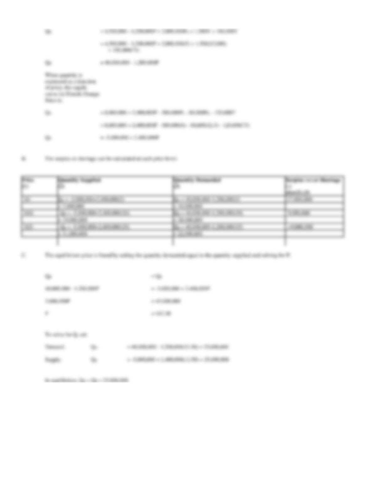
When quantity is expressed as a function of price, the demand curve for Florida Orange Juice is:
P
= $1 + $0.00002Q
Q
D.
Q
= QS + QC
To check, at P = $2:
Q
= 150,000
which is supported by the answer to part B, because QS + QC = 50,000 + 100,000 = 150,000.
50. Market Equilibrium. Various beverages are sold by roving vendors at Busch Stadium, home of the St.
Louis Cardinals. Demand and supply of the product are both highly sensitive to changes in the weather. During
hot summer months, demand for ice-cold beverages grows rapidly. On the other hand, hot dry weather has an
adverse effect on supply in that it taxes the stamina of the vendor carrying his or her goods up and down many
flights of stairs. The only competition for this service is provided by the beverages that can be purchased at
kiosks located throughout the stadium.
Demand and supply functions for ice-cold beverages per game are as follows:
QD
= 20,000 – 20,000P + 7,500PK + 0.8Y + 500T
(Demand)
QS
= 1,000 + 12,000P – 900PL – 1,000PC – 200T
(Supply)
where P is the average price of ice-cold beverage ($ per beverage), PK is the average price of beverages sold at the kiosks ($ per beverage), Y is
disposable income per household for baseball fans, T is the average daily high temperature (degrees), PL is the average price of unskilled labor ($ per
hour), and PC is the average cost of capital (in percent).
A.
When quantity is expressed as a function of price, what are the ice-cold beverage demand and supply curves if P = $5, PK = $4, Y =
$62,500, T = 80 degrees, PL = $10, and PC = 12%.
B.
Calculate the surplus or shortage of ice-cold beverage when P = $4, $5, and $6.
C.
Calculate the market equilibrium price-output combination.
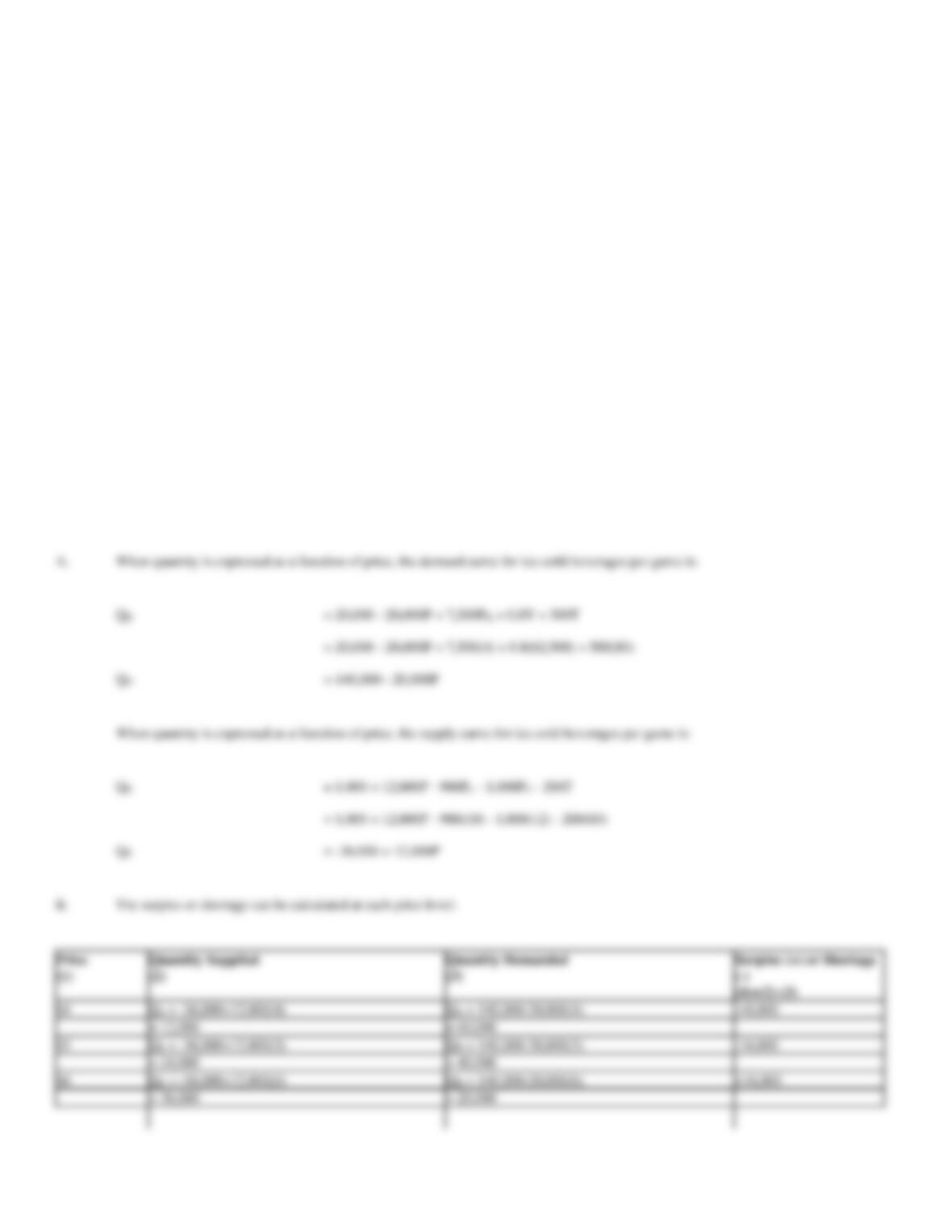
When quantity is expressed as a function of price, the demand curve for ice-cold beverages per game is:
QD
= 20,000 – 20,000P + 7,500PK + 0.8Y + 500T
= 20,000 – 20,000P + 7,500(4) + 0.8(62,500) + 500(80)
QD
= 140,000 – 20,000P
When quantity is expressed as a function of price, the supply curve for ice-cold beverages per game is:
QS
= 1,000 + 12,000P – 900PL – 1,000PC – 200T
= 1,000 + 12,000P – 900(10) – 1,000(12) – 200(80)
QS
QS = -36,000+12,000(4)
QD = 140,000-20,000(4)
-48,000
= 12,000
= 60,000
QS = -36,000+12,000(5)
QD = 140,000-20,000(5)
-16,000
= 24,000
= 40,000